Exercise 4
Questions
4.1 Estimate the Mincer equation of last weeks exercise seperately for East and West Germany for all years since 1992 using loops (see foreach).
4.2 Present the effects of years of education and of sex (the gender pay gap) graphically showing the trend since 1992 (see collapse) Tip: Use the Stata commands foreach, collapse and graph combine.
4.3 Tell Stata your data is panel data using xtset. Describe the variables of your Mincer equation and differentiate within and between variation (xtsum).
Data Prep
Stata
set more off
capt clear
version 14

use "_data/ex_mydf.dta", clear
. set more off

. capt clear

. version 14

.
. use "_data/ex_mydf.dta", clear
(PGEN: Feb 12, 2017 13:00:53-1 DBV32L)
R
#### load dataset ####
ex_mydf <- readRDS(file = "_data/ex_mydf.rds")

asample <- ex_mydf %>%
      filter(
            # Working Hours
            pgtatzeit >= 6,
            # age
            alter %>% dplyr::between(18, 65),
            # Employment Status
            pgemplst %in% c(1,2,4),   # full-time(1), part-time(2), marg.-empl(4)
            # population status
            pop < 3 # only private households
            ) %>%
      # filter unplausible cases
      mutate(na = case_when(
              pid %in% c(1380202, 1380202, 607602, 2555301) ~ 1,
              pid == 8267202 & syear == 2007 ~ 1,
              pid == 2633801 & syear == 2006 ~ 1,
              pid == 2582901 & syear > 2006 ~ 1 )
             ) %>%
      filter(is.na(na)) %>%
      # select relevant variables
      dplyr::select(hwageb, lnwage, pgbilzeit, cpgbilzeit, pgisco88, pgnace, pgexpue,
             sex, ost, erf, erfq, cerf, frau, pgallbet, phrf, syear, pid, pid_syear)
      # %>%
      # drop_na()
Answers
4.1 Mincer Equation
Estimate the Mincer equation of last weeks exercise seperately for East and West Germany for all years since 1992 using loops (see foreach).
Stata
use "_data/ex_mydf.dta", clear

cap drop educationrev
gen educationrev=.
cap drop upper lower
gen upper=.
gen lower=.

foreach year of numlist 1991/2015 {
      qui: reg lnwage pgbilzeit c.erf##c.erf pgexpue ost frau i.pgallbet if asample==1 & syear==`year' [pw=phrf], eform(b) cluster(hid)
      qui: replace educationrev = exp(_b[pgbilzeit]) if syear==`year'
      qui: replace upper = exp(_b[pgbilzeit]+ 1.96*_se[pgbilzeit]) if syear==`year'
      qui: replace lower = exp(_b[pgbilzeit]- 1.96*_se[pgbilzeit]) if syear==`year'
}

preserve
collapse educationrev upper lower, by(syear)
twoway (connected educationrev syear, sort) ///
(line upper lower syear, sort lpattern(dash dash) lcolor(bluishgray8 bluishgray8)) ///
, legend(off) subtitle(Gesamt)

graph save Graph "out/educationrev_gesamt.gph", replace
restore

** repeat for only West Germany

cap drop educationrev_west
gen educationrev_west =.
cap drop upper lower
gen upper=.
gen lower=.
foreach year of numlist 1984/2015 {
qui:  reg lnwage pgbilzeit c.erf##c.erf pgexpue ost frau i.pgallbet if asample==1 & syear==`year' & ost == 0 [pw=phrf], eform(b) cluster(hid)
qui: replace educationrev_west = exp(_b[pgbilzeit]) if syear==`year'
qui: replace upper = exp(_b[pgbilzeit]+ 1.96*_se[pgbilzeit]) if syear==`year'
qui: replace lower = exp(_b[pgbilzeit]- 1.96*_se[pgbilzeit]) if syear==`year'
}


preserve
collapse educationrev_west upper lower, by(syear)
twoway (connected educationrev_west syear, sort) ///
(line upper lower syear, sort lpattern(dash dash) lcolor(bluishgray8 bluishgray8)) ///
, legend(off) subtitle(West Germany)
graph save Graph "out/educationrev_west.gph", replace
restore


** repeat for only East Germany

cap drop educationrev_ost
gen educationrev_ost =.
cap drop upper lower
gen upper=.
gen lower=.
foreach year of numlist 1991/2015 {
qui: reg lnwage pgbilzeit c.erf##c.erf pgexpue ost frau i.pgallbet   if asample==1 & syear==`year' & ost == 1 [pw=phrf], eform(b) cluster(hid)
qui: replace educationrev_ost = exp(_b[pgbilzeit]) if syear==`year'
qui: replace upper = exp(_b[pgbilzeit]+ 1.96*_se[pgbilzeit]) if syear==`year'
qui: replace lower = exp(_b[pgbilzeit]- 1.96*_se[pgbilzeit]) if syear==`year'
}

preserve
collapse educationrev_ost upper lower, by(syear)
twoway (connected educationrev_ost syear, sort) ///
(line upper lower syear, sort lpattern(dash dash) lcolor(bluishgray8 bluishgray8)) ///
, legend(off) subtitle(East Germany)
graph save Graph "out/educationrev_ost.gph", replace
restore

***
graph combine  ///
      "out/educationrev_west.gph"  ///
      "out/educationrev_ost.gph"  ///
      "out/educationrev_gesamt.gph" ///
, ycommon xcommon note(GSOEP 32, size(vsmall) position(5)) title(Development of Education Returns)

graph save Graph "out/educationrev_all.gph", replace
. use "_data/ex_mydf.dta", clear
(PGEN: Feb 12, 2017 13:00:53-1 DBV32L)

.
. cap drop educationrev

. gen educationrev=.
(594,828 missing values generated)

. cap drop upper lower

. gen upper=.
(594,828 missing values generated)

. gen lower=.
(594,828 missing values generated)

.
. foreach year of numlist 1991/2015 {
  2.       qui: reg lnwage pgbilzeit c.erf##c.erf pgexpue ost frau i.pgallbet i
> f asample==1 & syear==`year' [pw=phrf], eform(b) cluster(hid)
  3.       qui: replace educationrev = exp(_b[pgbilzeit]) if syear==`year'
  4.       qui: replace upper = exp(_b[pgbilzeit]+ 1.96*_se[pgbilzeit]) if syea
> r==`year'
  5.       qui: replace lower = exp(_b[pgbilzeit]- 1.96*_se[pgbilzeit]) if syea
> r==`year'
  6. }

.
. preserve

. collapse educationrev upper lower, by(syear)

. twoway (connected educationrev syear, sort) ///
> (line upper lower syear, sort lpattern(dash dash) lcolor(bluishgray8 bluishgr
> ay8)) ///
> , legend(off) subtitle(Gesamt)

.
. graph save Graph "out/educationrev_gesamt.gph", replace
(file out/educationrev_gesamt.gph saved)

. restore

.
. ** repeat for only West Germany
.
. cap drop educationrev_west

. gen educationrev_west =.
(594,828 missing values generated)

. cap drop upper lower

. gen upper=.
(594,828 missing values generated)

. gen lower=.
(594,828 missing values generated)

. foreach year of numlist 1984/2015 {
  2. qui:  reg lnwage pgbilzeit c.erf##c.erf pgexpue ost frau i.pgallbet if asa
> mple==1 & syear==`year' & ost == 0 [pw=phrf], eform(b) cluster(hid)
  3. qui: replace educationrev_west = exp(_b[pgbilzeit]) if syear==`year'
  4. qui: replace upper = exp(_b[pgbilzeit]+ 1.96*_se[pgbilzeit]) if syear==`ye
> ar'
  5. qui: replace lower = exp(_b[pgbilzeit]- 1.96*_se[pgbilzeit]) if syear==`ye
> ar'
  6. }

.
.
. preserve

. collapse educationrev_west upper lower, by(syear)

. twoway (connected educationrev_west syear, sort) ///
> (line upper lower syear, sort lpattern(dash dash) lcolor(bluishgray8 bluishgr
> ay8)) ///
> , legend(off) subtitle(West Germany)

. graph save Graph "out/educationrev_west.gph", replace
(file out/educationrev_west.gph saved)

. restore

.
.
. ** repeat for only East Germany
.
. cap drop educationrev_ost

. gen educationrev_ost =.
(594,828 missing values generated)

. cap drop upper lower

. gen upper=.
(594,828 missing values generated)

. gen lower=.
(594,828 missing values generated)

. foreach year of numlist 1991/2015 {
  2. qui: reg lnwage pgbilzeit c.erf##c.erf pgexpue ost frau i.pgallbet   if as
> ample==1 & syear==`year' & ost == 1 [pw=phrf], eform(b) cluster(hid)
  3. qui: replace educationrev_ost = exp(_b[pgbilzeit]) if syear==`year'
  4. qui: replace upper = exp(_b[pgbilzeit]+ 1.96*_se[pgbilzeit]) if syear==`ye
> ar'
  5. qui: replace lower = exp(_b[pgbilzeit]- 1.96*_se[pgbilzeit]) if syear==`ye
> ar'
  6. }

.
. preserve

. collapse educationrev_ost upper lower, by(syear)

. twoway (connected educationrev_ost syear, sort) ///
> (line upper lower syear, sort lpattern(dash dash) lcolor(bluishgray8 bluishgr
> ay8)) ///
> , legend(off) subtitle(East Germany)

. graph save Graph "out/educationrev_ost.gph", replace
(file out/educationrev_ost.gph saved)

. restore

.
. ***
. graph combine  ///
>       "out/educationrev_west.gph"  ///
>       "out/educationrev_ost.gph"  ///
>       "out/educationrev_gesamt.gph" ///
> , ycommon xcommon note(GSOEP 32, size(vsmall) position(5)) title(Development
> of Education Returns)

.
. graph save Graph "out/educationrev_all.gph", replace
(file out/educationrev_all.gph saved)
R
Model
Trend by Year
# Fit Hourly Wage Brutto Model by year
      fit4.1 <- asample %>%
            group_by(syear) %>%
            do(model = lm(lnwage ~ 0+ pgbilzeit + I(erf^2) + pgexpue +
                                ost + frau + factor(pgallbet),
               data=., weights=phrf))
Trend by Year and Region
fit4.1_region <- asample %>%
      group_by(ost, syear) %>%
      do(model = lm(lnwage ~ 0 + pgbilzeit + I(erf^2) + pgexpue +
                          ost + frau + factor(pgallbet),
         data=., weights=phrf))

      # look at model
            # (fit4_region$model) # only use if not too many models
            #fit4_region %>% tidy(model)
            #fit4_region %>% glance(model)
            #fit4_region %>% augment(model)
Plot
Education Return Trend 1992 - 2015
     # grab relevant info
      td_fit <- fit4.1 %>% tidy(model, conf.int = TRUE)
      td_plot <- td_fit %>% filter(term == "pgbilzeit",
                                   syear > 1990)

      # Plot Over Years
      td_plot %>%
            ggplot(aes(x = syear, y = estimate)) +
            geom_point() +
            geom_errorbar(aes(ymin = conf.low, ymax = conf.high),
                          alpha=0.3, color = "black") +
            geom_line() +
            ylab("Education Return") +
            xlab("Survey Year") +
            ggtitle("Education Return from 1991 to 2015") +
            scale_x_continuous(breaks = seq(1991, 2016, by= 5))+
            scale_y_continuous(labels = scales::percent)+
            theme_bw()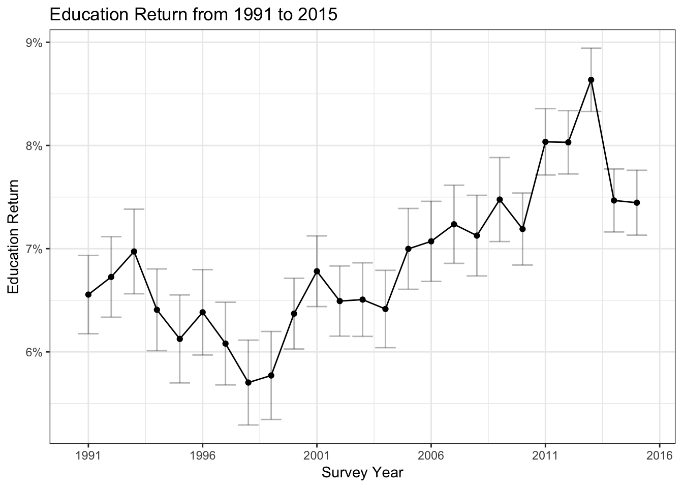
Education Return Trend over Time and Region
      # make tidy dataframe
      td_fit <- fit4.1_region %>% tidy(model, conf.int = TRUE)
      # select relevant info (coefficient for gender)
      td_plot <- td_fit %>% filter(term == "pgbilzeit")

      # plot Trend by Region (grouped)
      td_plot %>%
      ggplot(aes(x = syear, y = estimate,
                 color = as.factor(ost)), fill = as.factor(ost)) +
            geom_point() +
            geom_ribbon(ggplot2::aes_string(ymin = "conf.low", ymax = "conf.high",
                fill = "as.factor(ost)", color = NULL), alpha = 0.2) +
            geom_line() +
            ylab("Education Return") +
            xlab("Survey Year") +
            ggtitle("Education Return from 1984 to 2015 by Region") +
            scale_x_continuous(breaks = seq(1985, 2015, by= 5))+
            scale_y_continuous(labels = scales::percent)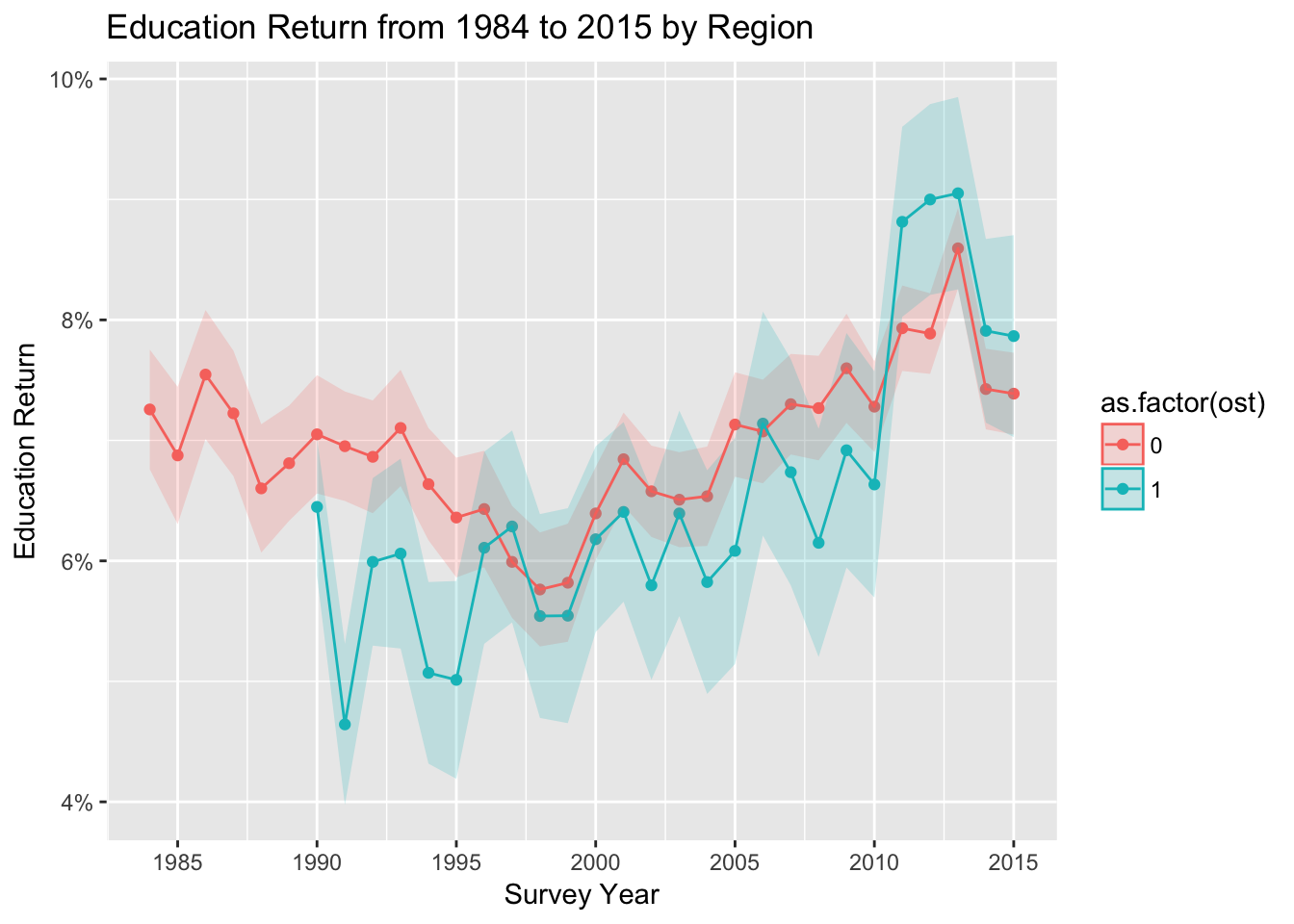
      # plot Trend by Region (facet)
      td_plot %>%
      ggplot(aes(x = syear, y = estimate)) +
            geom_point() +
            geom_errorbar(aes(ymin = conf.low, ymax = conf.high),
                          alpha=0.3, color = "black") +
            geom_line() +
            facet_wrap(~ ost)+
            ylab("Education Return") +
            xlab("Survey Year") +
            ggtitle("Education Return from 1984 to 2015 by Region") +
            scale_x_continuous(breaks = seq(1985, 2015, by= 5))+
            scale_y_continuous(labels = scales::percent)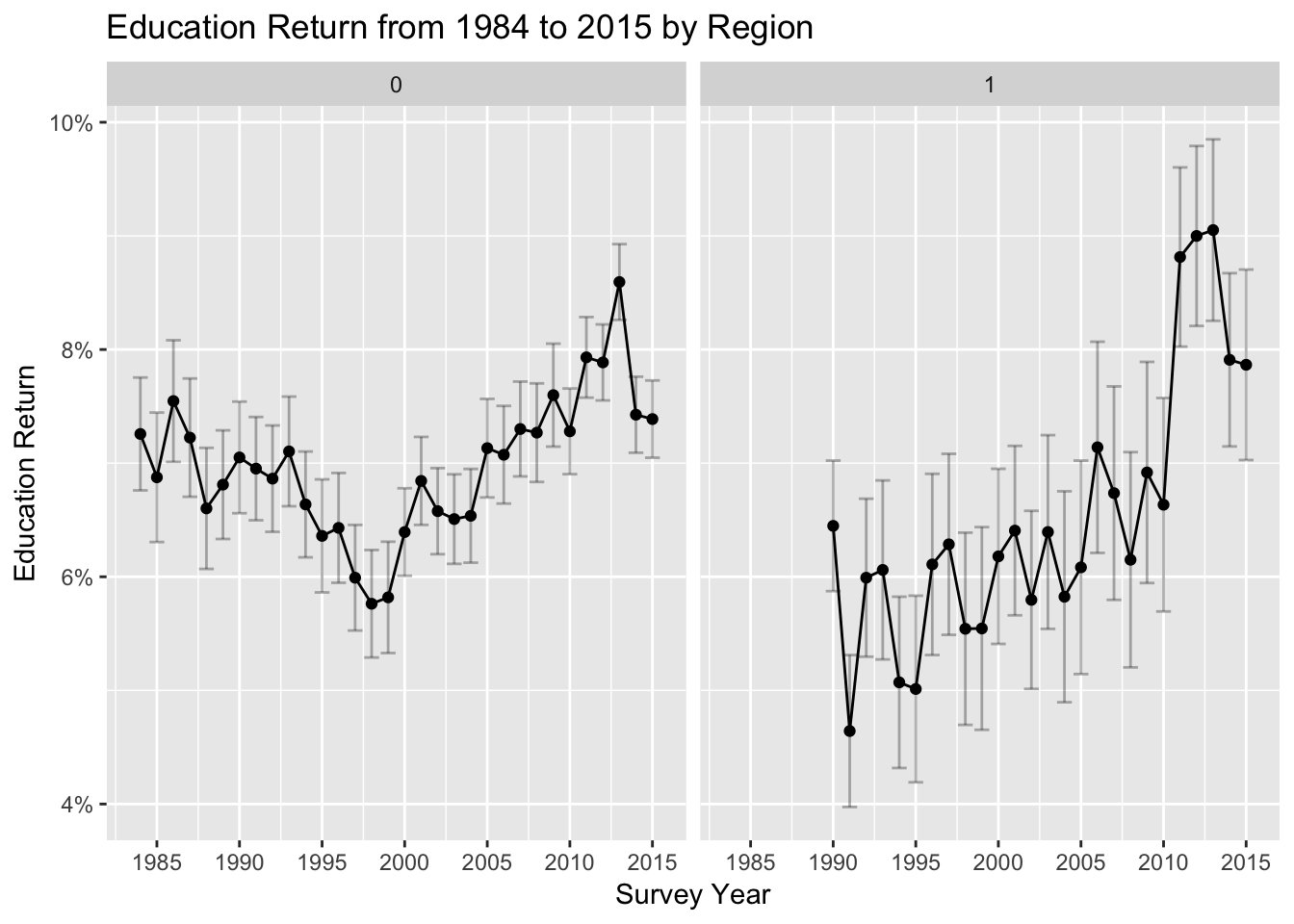
4.2 Gender Returns over Time
Present the effects of years of education and of sex (the gender pay gap) graphically showing the trend since 1992 (see collapse) Tip: Use the Stata commands foreach, collapse and graph combine.
Stata
use "_data/ex_mydf.dta", clear

cap drop genderrev
gen genderrev =.
cap drop upper lower
gen upper=.
gen lower=.

foreach year of numlist 1991/2015 {
      qui: reg lnwage pgbilzeit c.erf##c.erf pgexpue ost frau i.pgallbet if asample==1 & syear==`year' [pw=phrf], eform(b) cluster(hid)
      qui: replace genderrev = exp(_b[frau]) if syear==`year'
      qui: replace upper = exp(_b[frau]+ 1.96*_se[frau]) if syear==`year'
      qui: replace lower = exp(_b[frau]- 1.96*_se[frau]) if syear==`year'
}


preserve
collapse genderrev upper lower, by(syear)
twoway (connected genderrev syear, sort) ///
(line upper lower syear, sort lpattern(dash dash) lcolor(bluishgray8 bluishgray8)) ///
, legend(off) subtitle(Gesamt)
graph save Graph "out/genderrev_gesamt.gph", replace
restore

** repeat for only west germany
cap drop genderrev_west
gen genderrev_west=.
cap drop upper lower
gen upper=.
gen lower=.
foreach year of numlist 1984/2015 {
qui: reg lnwage frau c.erf##c.erf pgexpue ost frau i.pgallbet   if asample==1 & syear==`year' & ost==0 [pw=phrf], eform(b) cluster(hid)
qui: replace genderrev_west = exp(_b[frau]) if syear==`year'
qui: replace upper = exp(_b[frau]+ 1.96*_se[frau]) if syear==`year'
qui: replace lower = exp(_b[frau]- 1.96*_se[frau]) if syear==`year'
}
*twoway (connected genderrev_west syear, sort) (line upper lower syear, sort)
preserve
collapse genderrev_west upper lower, by(syear)
twoway (connected genderrev_west syear, sort) ///
(line upper lower syear, sort lpattern(dash dash) lcolor(bluishgray8 bluishgray8)) ///
, legend(off) subtitle(Ostdeutschland)
graph save Graph "out/genderrev_west.gph", replace
restore


** repeat for only east germany

cap drop genderrev_ost
gen genderrev_ost=.
cap drop upper lower
gen upper=.
gen lower=.
foreach year of numlist 1991/2015 {
qui: reg lnwage frau c.erf##c.erf pgexpue ost frau i.pgallbet   if asample==1 & syear==`year' & ost==1 [pw=phrf], eform(b) cluster(hid)
qui: replace genderrev_ost = exp(_b[frau]) if syear==`year'
qui: replace upper = exp(_b[frau]+ 1.96*_se[frau]) if syear==`year'
qui: replace lower = exp(_b[frau]- 1.96*_se[frau]) if syear==`year'
}
*twoway (connected genderrev_ost syear, sort) (line upper lower syear, sort)
preserve
collapse genderrev_ost upper lower, by(syear)
twoway (connected genderrev_ost syear, sort) ///
(line upper lower syear, sort lpattern(dash dash) lcolor(bluishgray8 bluishgray8)) ///
, legend(off) subtitle(Westdeutschland)
graph save Graph "out/genderrev_ost.gph", replace
restore

***
graph combine  ///
"out/genderrev_ost.gph"  ///
"out/genderrev_west.gph"  ///
"out/genderrev_gesamt.gph" ///
, ycommon xcommon note(GSOEP 32, size(vsmall) position(5)) title(Development of Gender Returns)

graph save Graph "out/genderrev_all.gph", replace
. use "_data/ex_mydf.dta", clear
(PGEN: Feb 12, 2017 13:00:53-1 DBV32L)

.
. cap drop genderrev

. gen genderrev =.
(594,828 missing values generated)

. cap drop upper lower

. gen upper=.
(594,828 missing values generated)

. gen lower=.
(594,828 missing values generated)

.
. foreach year of numlist 1991/2015 {
  2.       qui: reg lnwage pgbilzeit c.erf##c.erf pgexpue ost frau i.pgallbet i
> f asample==1 & syear==`year' [pw=phrf], eform(b) cluster(hid)
  3.       qui: replace genderrev = exp(_b[frau]) if syear==`year'
  4.       qui: replace upper = exp(_b[frau]+ 1.96*_se[frau]) if syear==`year'
  5.       qui: replace lower = exp(_b[frau]- 1.96*_se[frau]) if syear==`year'
  6. }

.
.
. preserve

. collapse genderrev upper lower, by(syear)

. twoway (connected genderrev syear, sort) ///
> (line upper lower syear, sort lpattern(dash dash) lcolor(bluishgray8 bluishgr
> ay8)) ///
> , legend(off) subtitle(Gesamt)

. graph save Graph "out/genderrev_gesamt.gph", replace
(file out/genderrev_gesamt.gph saved)

. restore

.
. ** repeat for only west germany
. cap drop genderrev_west

. gen genderrev_west=.
(594,828 missing values generated)

. cap drop upper lower

. gen upper=.
(594,828 missing values generated)

. gen lower=.
(594,828 missing values generated)

. foreach year of numlist 1984/2015 {
  2. qui: reg lnwage frau c.erf##c.erf pgexpue ost frau i.pgallbet   if asample
> ==1 & syear==`year' & ost==0 [pw=phrf], eform(b) cluster(hid)
  3. qui: replace genderrev_west = exp(_b[frau]) if syear==`year'
  4. qui: replace upper = exp(_b[frau]+ 1.96*_se[frau]) if syear==`year'
  5. qui: replace lower = exp(_b[frau]- 1.96*_se[frau]) if syear==`year'
  6. }

. *twoway (connected genderrev_west syear, sort) (line upper lower syear, sort)
>
. preserve

. collapse genderrev_west upper lower, by(syear)

. twoway (connected genderrev_west syear, sort) ///
> (line upper lower syear, sort lpattern(dash dash) lcolor(bluishgray8 bluishgr
> ay8)) ///
> , legend(off) subtitle(Ostdeutschland)

. graph save Graph "out/genderrev_west.gph", replace
(file out/genderrev_west.gph saved)

. restore

.
.
. ** repeat for only east germany
.
. cap drop genderrev_ost

. gen genderrev_ost=.
(594,828 missing values generated)

. cap drop upper lower

. gen upper=.
(594,828 missing values generated)

. gen lower=.
(594,828 missing values generated)

. foreach year of numlist 1991/2015 {
  2. qui: reg lnwage frau c.erf##c.erf pgexpue ost frau i.pgallbet   if asample
> ==1 & syear==`year' & ost==1 [pw=phrf], eform(b) cluster(hid)
  3. qui: replace genderrev_ost = exp(_b[frau]) if syear==`year'
  4. qui: replace upper = exp(_b[frau]+ 1.96*_se[frau]) if syear==`year'
  5. qui: replace lower = exp(_b[frau]- 1.96*_se[frau]) if syear==`year'
  6. }

. *twoway (connected genderrev_ost syear, sort) (line upper lower syear, sort)
. preserve

. collapse genderrev_ost upper lower, by(syear)

. twoway (connected genderrev_ost syear, sort) ///
> (line upper lower syear, sort lpattern(dash dash) lcolor(bluishgray8 bluishgr
> ay8)) ///
> , legend(off) subtitle(Westdeutschland)

. graph save Graph "out/genderrev_ost.gph", replace
(file out/genderrev_ost.gph saved)

. restore

.
. ***
. graph combine  ///
> "out/genderrev_ost.gph"  ///
> "out/genderrev_west.gph"  ///
> "out/genderrev_gesamt.gph" ///
> , ycommon xcommon note(GSOEP 32, size(vsmall) position(5)) title(Development
> of Gender Returns)

.
. graph save Graph "out/genderrev_all.gph", replace
(file out/genderrev_all.gph saved)

.
R
Model
The Plots are based on the same models as in 4.1.
Plot
Gender Return Trend 1991 - 2015
     # grab relevant info
      td_fit <- fit4.1 %>% tidy(model, conf.int = TRUE)
      td_plot <- td_fit %>% filter(term == "frau",
                                   syear > 1990)

      # Plot Over Years
      td_plot %>%
            ggplot(aes(x = syear, y = estimate)) +
            geom_point() +
            geom_errorbar(aes(ymin = conf.low, ymax = conf.high),
                          alpha=0.3, color = "black") +
            geom_line() +
            ylab("Gender Return") +
            xlab("Survey Year") +
            ggtitle("Gender Pay Gap from 1991 to 2015") +
            scale_x_continuous(breaks = seq(1991, 2016, by= 5))+
            scale_y_reverse(labels = scales::percent)+
            theme_bw()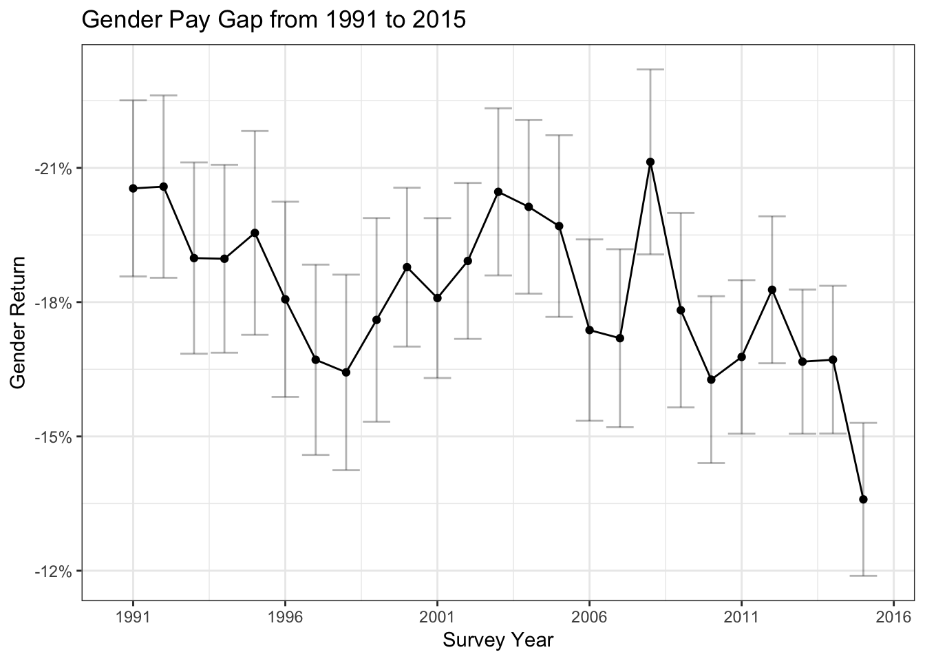
Gender Return Trend by Year and Gender
      # make tidy dataframe
      td_fit <- fit4.1_region %>% tidy(model, conf.int = TRUE)
      # select relevant info (coefficient for gender)
      td_plot <- td_fit %>% filter(term == "frau")

      # plot Trend by Region (grouped)
      td_plot %>%
      ggplot(aes(x = syear, y = estimate, color = as.factor(ost))) +
            geom_point() +
            geom_errorbar(aes(ymin = conf.low, ymax = conf.high),
                          alpha=0.3, color = "black") +
            geom_line() +
            ylab("Gender Return") +
            xlab("Survey Year") +
            ggtitle("Gender Pay Gap by Region") +
            scale_x_continuous(breaks = seq(1985, 2015, by= 5))+
            scale_y_reverse(labels = scales::percent)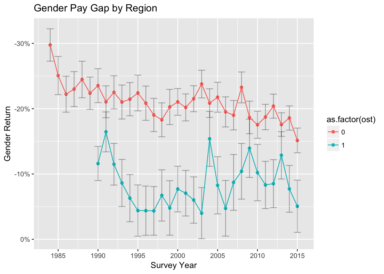
      # plot Trend by Region (facet)
      td_plot %>%
      ggplot(aes(x = syear, y = estimate)) +
            geom_point() +
            geom_errorbar(aes(ymin = conf.low, ymax = conf.high),
                          alpha=0.3, color = "black") +
            geom_line() +
            facet_wrap(~ost)+
            ylab("Gender Return") +
            xlab("Survey Year") +
            ggtitle("Gender Pay Gap by Region") +
            scale_x_continuous(breaks = seq(1985, 2015, by= 5))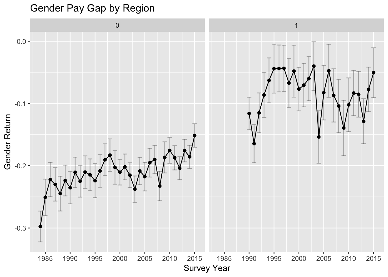
4.3 xtset
Tell Stata your data is panel data using xtset. Describe the variables of your Mincer equation and differentiate within and between variation (xtsum).
Note: STATA within min and max: in order to get the correct min and max of the person specific within standard deviations in STATA, you have to subtract / add the grand mean to the displayed values
Stata
use "_data/ex_mydf.dta", clear

*tab pop
*tab pgstib

*Only private Households (pop > 3), not in wf (10), apprentice (11), unempl (12), retired (13)
cap drop asample
gen asample = 1 if pop < 3 & pgstib!=10 & pgstib!=11 & pgstib!=12 & pgstib != 13

xtset pid syear
*xtdes

xtreg lnwage c.erf##c.erf pgexpue frau i.pgallbet if asample==1, fe

* xtsum
xtsum lnwage pgbilzeit erf ost frau if asample==1

*** Tabellen
xttab
. use "_data/ex_mydf.dta", clear
(PGEN: Feb 12, 2017 13:00:53-1 DBV32L)

.
. *tab pop
. *tab pgstib
.
. *Only private Households (pop > 3), not in wf (10), apprentice (11), unempl (
> 12), retired (13)
. cap drop asample

. gen asample = 1 if pop < 3 & pgstib!=10 & pgstib!=11 & pgstib!=12 & pgstib !=
>  13
(240,353 missing values generated)

.
. xtset pid syear
       panel variable:  pid (unbalanced)
        time variable:  syear, 1984 to 2015, but with gaps
                delta:  1 unit

. *xtdes
.
. xtreg lnwage c.erf##c.erf pgexpue frau i.pgallbet if asample==1, fe
note: frau omitted because of collinearity

Fixed-effects (within) regression               Number of obs     =    311,775
Group variable: pid                             Number of groups  =     50,711

R-sq:                                           Obs per group:
     within  = 0.0952                                         min =          1
     between = 0.2687                                         avg =        6.1
     overall = 0.1958                                         max =         32

                                                F(7,261057)       =    3925.97
corr(u_i, Xb)  = -0.0184                        Prob > F          =     0.0000

------------------------------------------------------------------------------
      lnwage |      Coef.   Std. Err.      t    P>|t|     [95% Conf. Interval]
-------------+----------------------------------------------------------------
         erf |   .0594265   .0004077   145.77   0.000     .0586275    .0602255
             |
 c.erf#c.erf |   -.000997   9.51e-06  -104.88   0.000    -.0010156   -.0009783
             |
     pgexpue |  -.0302878   .0014773   -20.50   0.000    -.0331834   -.0273922
        frau |          0  (omitted)
             |
    pgallbet |
[2] GE 20..  |   .0574398   .0029346    19.57   0.000      .051688    .0631915
[3] GE 20..  |   .0954839   .0034194    27.92   0.000     .0887819    .1021859
[4] GE 2000  |   .1131657   .0036127    31.32   0.000     .1060848    .1202465
[5] Selbs..  |  -.0302114   .0059587    -5.07   0.000    -.0418902   -.0185326
             |
       _cons |   1.949638    .004002   487.16   0.000     1.941794    1.957482
-------------+----------------------------------------------------------------
     sigma_u |   .5570618
     sigma_e |  .36230039
         rho |  .70274527   (fraction of variance due to u_i)
------------------------------------------------------------------------------
F test that all u_i=0: F(50710, 261057) = 9.88               Prob > F = 0.0000

.
. * xtsum
. xtsum lnwage pgbilzeit erf ost frau if asample==1

Variable         |      Mean   Std. Dev.       Min        Max |    Observations
-----------------+--------------------------------------------+----------------
lnwage   overall |  2.556967   .6522679  -5.025553   7.214181 |     N =  328322
         between |             .6568632  -4.962845   6.289409 |     n =   56025
         within  |             .3543293  -4.673269   6.503639 | T-bar = 5.86028
                 |                                            |
pgbilz~t overall |  12.18844   2.734574          7         18 |     N =  341889
         between |             2.669908          7         18 |     n =   56309
         within  |             .5543849    1.92177    20.3551 | T-bar = 6.07166
                 |                                            |
erf      overall |  16.05425   11.56454          0      64.48 |     N =  344352
         between |              11.8974          0   63.85333 |     n =   53729
         within  |             3.899642  -.1444556   35.28363 | T-bar = 6.40905
                 |                                            |
ost      overall |  .2085112   .4062447          0          1 |     N =  354475
         between |             .3907451          0          1 |     n =   60394
         within  |             .0676974  -.7498222   1.177261 | T-bar = 5.86937
                 |                                            |
frau     overall |  .4573637   .4981795          0          1 |     N =  354475
         between |             .4996421          0          1 |     n =   60394
         within  |                    0   .4573637   .4573637 | T-bar = 5.86937

.
. *** Tabellen
. xttab
varlist required
r(100);

end of do-file
r(100);
R
In R there is no package available that calculates the between and within variance of variables in panel datasets. Therefore we need to write a function to achieve the desired goal. The function used in this case originates from here and has been adapted a bit.
In a first step the overall descriptive statistics are calculated and stored, then the between means are calculated for each individual and then the variation and other statistics are calculated. Lastly the stats for within variation are calculated and the stored results are returned. The function can now be used in the following way:
The function XTSUM takes three inputs:
data – the dataset varname – the variable to xtsum unit – the identifier for the within dimension
asample <- ex_mydf %>%
      filter(
            # only private households
            pop <= 2,
            # only workforce
            # not in wf (10), apprentice (11), unempl (12), retired (13)
            !pgstib %in% c(10,11,12,13)
      )

# quick frequency table
# asample %>% group_by(syear) %>% summarise(n = n()) %>% as.data.frame()

XTSUM <- function(data, varname, unit) {
  varname <- enquo(varname)
  loc.unit <- enquo(unit)

ores <- data %>% summarise(ovr.mean = mean(!! varname, na.rm=TRUE),
                           ovr.sd = sd(!! varname, na.rm=TRUE),
                           ovr.min = min(!! varname, na.rm=TRUE),
                           ovr.max = max(!! varname, na.rm=TRUE),
                           ovr.N = sum(as.numeric((!is.na(!! varname)))),
                           ovr.N2 = n())
bmeans <- data %>%
      group_by(!! loc.unit) %>%
      summarise(meanx = mean(!! varname, na.rm=T),
                t.count = sum(as.numeric(!is.na(!! varname))),
                t.count2 = na.omit(n())
                )


bres <- bmeans %>%
      ungroup() %>%
      summarise(between.sd = sd(meanx, na.rm=TRUE),
                between.min = min(meanx, na.rm=TRUE),
                between.max = max(meanx, na.rm=TRUE),
                Units = sum(as.numeric(!is.na(t.count))),
                t.bar = mean(t.count, na.rm=TRUE),
                t.bar2 = mean(t.count2, na.rm = T))

wdat <- data %>%
      group_by(!! loc.unit) %>%
      mutate(W.x = scale(!! varname, scale=FALSE))

wres <- wdat %>%
      ungroup() %>%
      summarise(within.sd = sd(W.x, na.rm=TRUE),
                within.min = min(W.x, na.rm=TRUE),
                within.max = max(W.x, na.rm=TRUE))

return(list(ores = ores, bres = bres, wres = wres))
}
Using the function
XTSUM(asample, varname = lnwage , unit = pid)## $ores
## # A tibble: 1 x 5
## ovr.mean ovr.sd ovr.min ovr.max ovr.N
## <dbl> <dbl> <dbl> <dbl> <dbl>
## 1 2.16 0.764 -5.28 7.03 332797
##
## $bres
## # A tibble: 1 x 5
## between.sd between.min between.max Units t.bar
## <dbl> <dbl> <dbl> <dbl> <dbl>
## 1 0.755 -4.96 6.03 95777 3.47
##
## $wres
## # A tibble: 1 x 3
## within.sd within.min within.max
## <dbl> <dbl> <dbl>
## 1 0.446 -6.99 4.13XTSUM(asample, varname = pgbilzeit , unit = pid)## $ores
## # A tibble: 1 x 5
## ovr.mean ovr.sd ovr.min ovr.max ovr.N
## <dbl> <dbl> <dbl> <dbl> <dbl>
## 1 12.2 2.73 7.00 18.0 341889
##
## $bres
## # A tibble: 1 x 5
## between.sd between.min between.max Units t.bar
## <dbl> <dbl> <dbl> <dbl> <dbl>
## 1 2.67 7.00 18.0 95777 3.57
##
## $wres
## # A tibble: 1 x 3
## within.sd within.min within.max
## <dbl> <dbl> <dbl>
## 1 0.554 -10.3 8.17XTSUM(asample, varname = frau , unit = pid)## $ores
## # A tibble: 1 x 5
## ovr.mean ovr.sd ovr.min ovr.max ovr.N
## <dbl> <dbl> <dbl> <dbl> <dbl>
## 1 0.464 0.499 0 1.00 575397
##
## $bres
## # A tibble: 1 x 5
## between.sd between.min between.max Units t.bar
## <dbl> <dbl> <dbl> <dbl> <dbl>
## 1 0.500 0 1.00 95777 6.01
##
## $wres
## # A tibble: 1 x 3
## within.sd within.min within.max
## <dbl> <dbl> <dbl>
## 1 0 0 0XTSUM(asample, varname = pgallbet , unit = pid)## $ores
## # A tibble: 1 x 5
## ovr.mean ovr.sd ovr.min ovr.max ovr.N
## <dbl> <dbl> <dbl> <dbl> <dbl>
## 1 2.49 1.20 1.00 5.00 333299
##
## $bres
## # A tibble: 1 x 5
## between.sd between.min between.max Units t.bar
## <dbl> <dbl> <dbl> <dbl> <dbl>
## 1 1.08 1.00 5.00 95777 3.48
##
## $wres
## # A tibble: 1 x 3
## within.sd within.min within.max
## <dbl> <dbl> <dbl>
## 1 0.680 -3.88 3.88XTSUM(asample, varname = pgexpue , unit = pid)## $ores
## # A tibble: 1 x 5
## ovr.mean ovr.sd ovr.min ovr.max ovr.N
## <dbl> <dbl> <dbl> <dbl> <dbl>
## 1 0.489 1.46 0 34.3 344352
##
## $bres
## # A tibble: 1 x 5
## between.sd between.min between.max Units t.bar
## <dbl> <dbl> <dbl> <dbl> <dbl>
## 1 1.68 0 34.3 95777 3.60
##
## $wres
## # A tibble: 1 x 3
## within.sd within.min within.max
## <dbl> <dbl> <dbl>
## 1 0.488 -11.5 14.1further Links on this topic: - https://stackoverflow.com/questions/14165752/between-within-standard-deviations-in-r - https://www.r-bloggers.com/dplyr-do-some-tips-for-using-and-programming/ - psdata: https://github.com/rOpenGov/psData/issues/5 - dplyr xtsum: https://github.com/hadley/vctrs/issues/17 - https://christophergandrud.github.io/RepResR-RStudio/ - Get the column number in R given the column name - which( colnames(df)==“b” ) - https://stackoverflow.com/questions/16367436/compute-mean-and-standard-deviation-by-group-for-multiple-variables-in-a-data-fr