Exercise 3
Questions
3.1 You should start with an income equation with hourly gross wages (do not use the log-transfromation for now). Predictor variables are years of education, labor force experience, sex and region.
3.2 Specify an interaction effect for sex and years of education. Interpret the results.
3.3 Present your results grafically using a marginal effects plot
3.4 Specify another interaction effect between years of education and labor force experience. Interpret the results. Use a marginal effects plot to do that.
3.5 Include a nominal (e. g. company size: pgallbet) variable with more than two categories as predictors using a dummy set.
3.6 Drop the interactions and the dummy set. Include duration of unemployment as additional predictor. What has the largest effect, years of education, labor force experience or duration of unemployment?
3.7 Specify a quadratic effect for labor force participation. Interpret the result using a marginal effects plot.
3.8 Now, use log-transformed income as dependent variable. Interpret the effect of years of education on income. Present your result in a table using estout or esttab.
Data Prep
Stata
set more off
capt clear
version 14

use "_data/ex_mydf.dta", clear
. set more off

. capt clear

. version 14

.
. use "_data/ex_mydf.dta", clear
(PGEN: Feb 12, 2017 13:00:53-1 DBV32L)
R
Load Data
#### load dataset ####
ex_mydf <- readRDS(file = "_data/ex_mydf.rds")

asample <- ex_mydf %>%
        filter(pgtatzeit > 5,
               alter %>% dplyr::between(18, 65),
               pgemplst %in% c(1,2,4),
               pop<3
               ) %>%
      # filter unplausible cases
      mutate(na = case_when(
              pid %in% c(1380202, 1380202, 607602, 2555301) ~ 1,
              pid == 8267202 & syear == 2007 ~ 1,
              pid == 2633801 & syear == 2006 ~ 1,
              pid == 2582901 & syear > 2006 ~ 1 )
             ) %>%
      filter(is.na(na)) %>%
      select(hwageb, lnwage, pgbilzeit, cpgbilzeit, erf, cerf, erfq, pgexpue, frau, ost, phrf, syear )

## Sample For Analysis for 2015
asample15 <- asample %>% filter(syear == 2015)
Answers
3.1 Basic Model
You should start with an income equation with hourly gross wages hwageb (do not use the log-transfromation for now). Predictor variables are years of education pgbilzeit, labor force experience erf, sex frau and region ost.
Stata
use "_data/ex_mydf.dta", clear

reg hwageb pgbilzeit erf frau ost if asample==1 & syear==2015 [pw=phrf]
. use "_data/ex_mydf.dta", clear
(PGEN: Feb 12, 2017 13:00:53-1 DBV32L)

.
. reg hwageb pgbilzeit erf frau ost if asample==1 & syear==2015 [pw=phrf]
(sum of wgt is   3.3886e+07)

Linear regression                               Number of obs     =     14,218
                                                F(4, 14213)       =     259.84
                                                Prob > F          =     0.0000
                                                R-squared         =     0.2253
                                                Root MSE          =     10.072

------------------------------------------------------------------------------
             |               Robust
      hwageb |      Coef.   Std. Err.      t    P>|t|     [95% Conf. Interval]
-------------+----------------------------------------------------------------
   pgbilzeit |   1.638184   .0619018    26.46   0.000     1.516848     1.75952
         erf |   .2431915   .0109426    22.22   0.000     .2217425    .2646405
        frau |  -2.754198   .2425546   -11.35   0.000    -3.229636   -2.278759
         ost |  -4.278906   .2718054   -15.74   0.000     -4.81168   -3.746132
       _cons |  -6.573576   .7699179    -8.54   0.000    -8.082716   -5.064436
------------------------------------------------------------------------------
R
version 1
Overview of model with summary()
fit3.1  <- asample15 %>%
            lm(hwageb~ pgbilzeit + erf + ost + frau, data=., weights=phrf)

summary(fit3.1)
##
## Call:
## lm(formula = hwageb ~ pgbilzeit + erf + ost + frau, data = .,
## weights = phrf)
##
## Weighted Residuals:
## Min 1Q Median 3Q Max
## -2648 -150 -15 118 19905
##
## Coefficients:
## Estimate Std. Error t value Pr(>|t|)
## (Intercept) -6.57538 0.46397 -14.2 <2e-16 ***
## pgbilzeit 1.63828 0.03102 52.8 <2e-16 ***
## erf 0.24324 0.00762 31.9 <2e-16 ***
## ost -4.28070 0.22214 -19.3 <2e-16 ***
## frau -2.75467 0.17368 -15.9 <2e-16 ***
## ---
## Signif. codes: 0 '***' 0.001 '**' 0.01 '*' 0.05 '.' 0.1 ' ' 1
##
## Residual standard error: 492 on 14216 degrees of freedom
## (549 observations deleted due to missingness)
## Multiple R-squared: 0.226, Adjusted R-squared: 0.225
## F-statistic: 1.04e+03 on 4 and 14216 DF, p-value: <2e-16version 2
Overview of model with tidy() and glance() fro the broom package. glance()gives an overview of the general model, while tidy() shows the results of the model and confidence intervals (those are optional).
# overall model
glance(fit3.1)
# model coefficients
tidy(fit3.1, conf.int = T)3.2 Interaction
Specify an interaction effect for sex and years of education. Interpret the results.
In the prior model, with only main effects, we could interpret the gender variable frau as the difference between females (1) and males (0). Now that we added the interaction term, we allow the slopes for years of education to differ between females and males. The presence of the interaction implies that the effect of education depends on the gender of a person. The term frau:pgbilzeit indicates the extend to which the difference between females and males changes for every year of education. The coefficient for years of education pgbilzeit indicates the effect of education on hourly wages for males (reference category: frau == 0). The model predicts, that for every increase of education by one unit (year), hourly wage increases by 1.84 € for males and by 1.84 € - 0.46 € = 1.38 € for females (all other factors held constant).
This is visualized in the following plots of exercise 3.3.
Stata
use "_data/ex_mydf.dta", clear

reg hwageb i.frau##c.pgbilzeit erf ost if asample==1 & syear==2015 [pw=phrf]
. use "_data/ex_mydf.dta", clear
(PGEN: Feb 12, 2017 13:00:53-1 DBV32L)

.
. reg hwageb i.frau##c.pgbilzeit erf ost if asample==1 & syear==2015 [pw=phrf]
(sum of wgt is   3.3886e+07)

Linear regression                               Number of obs     =     14,218
                                                F(5, 14212)       =     266.80
                                                Prob > F          =     0.0000
                                                R-squared         =     0.2284
                                                Root MSE          =     10.053

------------------------------------------------------------------------------
             |               Robust
      hwageb |      Coef.   Std. Err.      t    P>|t|     [95% Conf. Interval]
-------------+----------------------------------------------------------------
        frau |
   weiblich  |    3.14171   1.351724     2.32   0.020     .4921544    5.791265
   pgbilzeit |    1.84609   .0991546    18.62   0.000     1.651734    2.040446
             |
        frau#|
 c.pgbilzeit |
   weiblich  |  -.4573853   .1146227    -3.99   0.000    -.6820608   -.2327097
             |
         erf |   .2446797    .010997    22.25   0.000      .223124    .2662353
         ost |  -4.236248    .269402   -15.72   0.000    -4.764311   -3.708184
       _cons |  -9.272963   1.208191    -7.68   0.000    -11.64117   -6.904751
------------------------------------------------------------------------------
R
fit3.2 <- asample15 %>%
      select(hwageb, pgbilzeit, frau, erf, ost, phrf) %>%
      drop_na %>%
      lm(hwageb ~ frau*pgbilzeit + erf + ost, data= ., weights = phrf)

# overall model
glance(fit3.2)
# model coefficients
tidy(fit3.2, conf.int = T)3.3 Marginal Effects
Present your results grafically using a marginal effects plot.
Stata
knitr::include_graphics("out/margins_3_3.png")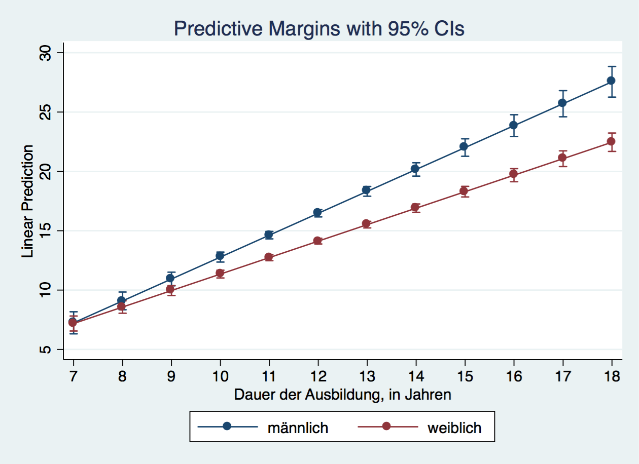
use "_data/ex_mydf.dta", clear

reg hwageb i.frau##c.pgbilzeit erf ost if asample==1 & syear==2015 [pw=phrf]

qui: margins, at(pgbilzeit=(7 (1) 18) frau=(1 0))
marginsplot, name(margins_3_3, replace)

graph use margins_3_3
graph export "out/margins_3_3_text.png", replace
R
Plots
Marginsplot
two versions, the first one more fancy code, the second a quick alternative. An alternative way to model marginal effects is the marginspackage.
# Marginsplot for Years of Education and Gender
 dat <- ggpredict(fit3.2, terms = c("pgbilzeit", "frau"))

# fancy plot
 ggplot(dat, aes(x, predicted, color = group, fill = group)) +
       geom_line()+
       geom_point()+
       geom_ribbon(ggplot2::aes_string(ymin = "conf.low",
                ymax = "conf.high", color = NULL), alpha = 0.25) +
       labs(x = get_x_title(dat), y = get_y_title(dat))+
       ggtitle("Predicted Values for Hourly Wages in Prices of 2015")+
       guides(fill = guide_legend(title="Gender"),color = F)+
       theme(legend.position="bottom")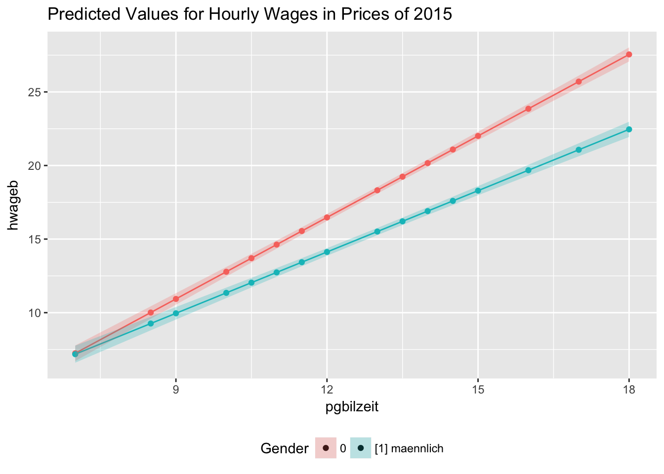
# quick alternative
 plot(dat)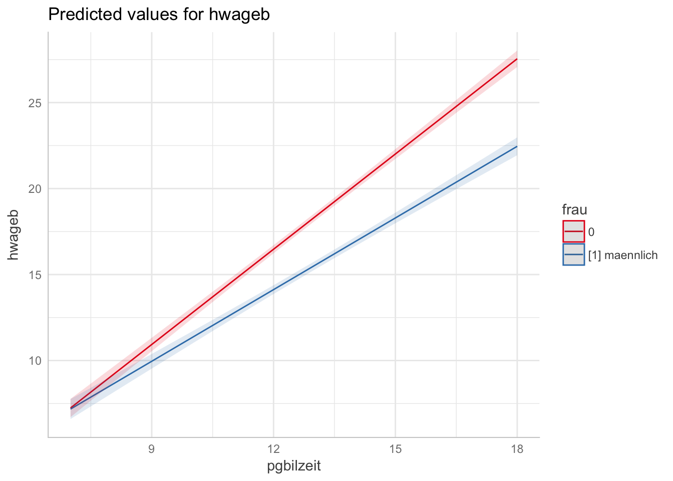
Coeff-Plots
The following plots are created with interplot(). The plot showa the distribution of coefficients of var1 conditional on values of var2. E.g. if we intend to know how the coefficients for years of education and gender are related, var1 could be years of education pgbilzeit while var2 is gender frau. One feature that I like about these plots is that yu can also specify a histoption in order to add the distribution of the variable who`s coefficients are being plottet. The negative slope of the gender coefficient with increasing years of education, shows that with increasing years of education, the magnitude of the gender wage gap increases.
# interplot notes:
# m = the object of a regression result
# var1 = var whose coefficient is to be plotted
# var2 = var on which the coefficient is conditional (var2)

# parameters:   point = wether a line or points are shown
#               hist = it can be helpful to the evaluation of the substantive significance of the conditional effect to know the distribution of the conditioning variable (years of education)

interplot(m = fit3.2 , var1 = "frau", var2= "pgbilzeit", point = F, hist = T) +
            theme(axis.text.x  = element_text(angle=45)) +
            xlab("Education (in years)") +
            ylab("Estimated Coefficient for\nGender") +
            ggtitle("Coefficients of Gender by Years of Education") +
            theme(plot.title = element_text(face="bold")) +
            # Add a horizontal line at y = 0
            geom_hline(yintercept = 0, linetype = "dashed")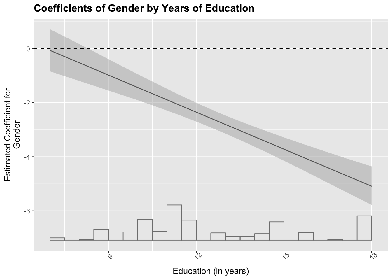
interplot(m = fit3.2 ,var1 = "pgbilzeit" , var2="frau")+
            ggtitle("Coefficients of Education by Gender")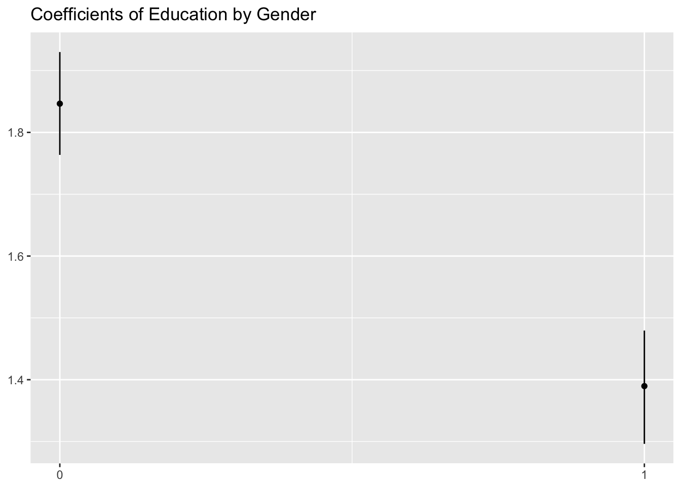
3.4 Interaction II
Specify another interaction effect between years of education and labor force experience. Interpret the results. Use a marginal effects plot to do that.
One can see in the marginsplot that the predicted hourly wage for the different values of years of work experience has different slopes depending on years of education. While there is almost no change in wage due to work experience for little education (e.g.7 yrs) the positive effect of work experience increases as years of education increase.
Stata
Model
Two way interactions gender:education education:workexperience
use "_data/ex_mydf.dta", clear

reg hwageb i.frau##c.pgbilzeit c.pgbilzeit##c.erf ost if asample==1 & syear==2015 [pw=phrf]

qui: margins, at(erf=(0(10)50) pgbilzeit=(7, 10.5, 14, 18)
marginsplot, name(margins_3_4, replace)

graph use margins_3_4
graph export "out/margins_3_4.png"
. use "_data/ex_mydf.dta", clear
(PGEN: Feb 12, 2017 13:00:53-1 DBV32L)

.
. reg hwageb i.frau##c.pgbilzeit c.pgbilzeit##c.erf ost if asample==1 & syear==
> 2015 [pw=phrf]
(sum of wgt is   3.3886e+07)
note: pgbilzeit omitted because of collinearity

Linear regression                               Number of obs     =     14,218
                                                F(6, 14211)       =     247.98
                                                Prob > F          =     0.0000
                                                R-squared         =     0.2391
                                                Root MSE          =     9.9834

------------------------------------------------------------------------------
             |               Robust
      hwageb |      Coef.   Std. Err.      t    P>|t|     [95% Conf. Interval]
-------------+----------------------------------------------------------------
        frau |
   weiblich  |   .6040457     1.3138     0.46   0.646    -1.971175    3.179267
   pgbilzeit |   1.117752   .1180213     9.47   0.000     .8864144    1.349089
             |
        frau#|
 c.pgbilzeit |
   weiblich  |  -.2616283   .1115297    -2.35   0.019    -.4802412   -.0430155
             |
   pgbilzeit |          0  (omitted)
         erf |  -.2539583   .0644679    -3.94   0.000    -.3803239   -.1275927
             |
 c.pgbilzeit#|
       c.erf |   .0398017   .0056076     7.10   0.000     .0288101    .0507932
             |
         ost |  -4.415959   .2691979   -16.40   0.000    -4.943622   -3.888296
       _cons |   .1061027   1.392269     0.08   0.939    -2.622927    2.835132
------------------------------------------------------------------------------

.
. qui: margins, at(erf=(0(10)50) pgbilzeit=(7, 10.5, 14, 18)
) required
r(100);

end of do-file
r(100);
Plot
two interactions
knitr::include_graphics("out/margins_3_4.png")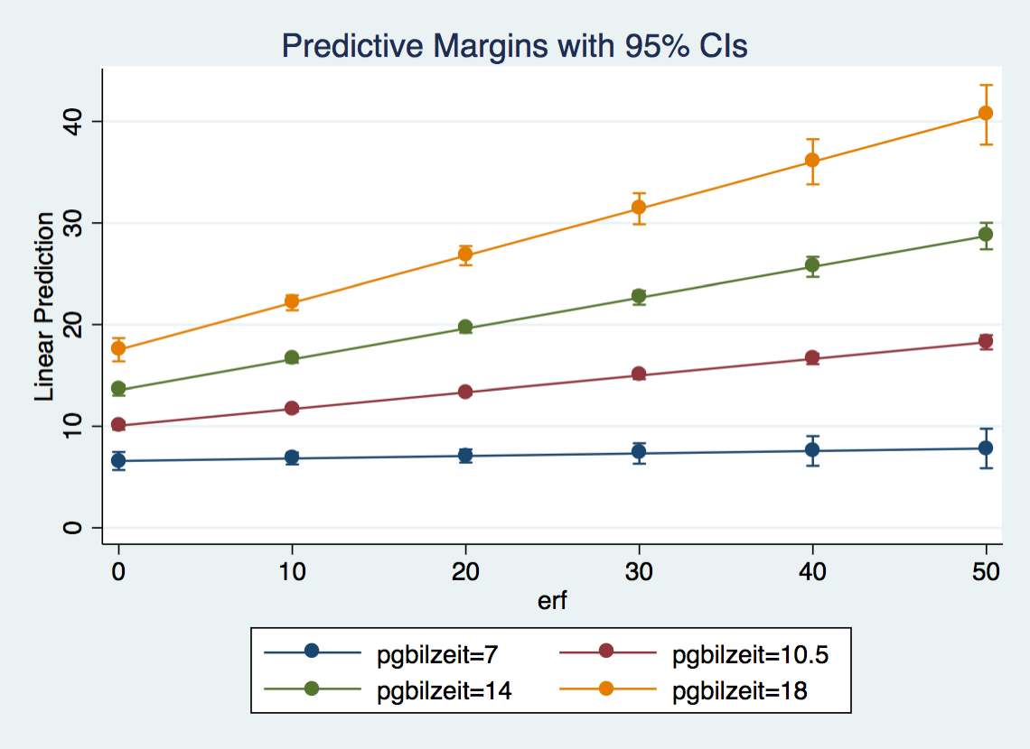
R
Model
Fit 3.4
fit3.4 <- asample15 %>%
      lm(hwageb ~ frau*pgbilzeit + pgbilzeit*erf + ost,
         data = ., weights = phrf)

tidy(fit3.4, conf.int = T)glance(fit3.4)Plots
Marginal Effect Plot
Marginsplot for Years of Education and Work Experience
 dat <- ggpredict(fit3.4, terms = c("erf [0,10,20,30,40,50]", "pgbilzeit [7,10.5,14,18]"))

 ggplot(dat, aes(x, predicted, color = group, fill = group)) +
       geom_point()+
       geom_line()+
      geom_ribbon(ggplot2::aes_string(ymin = "conf.low",
                ymax = "conf.high", color = NULL), alpha = 0.25)+
       labs(x = get_x_title(dat), y = get_y_title(dat))+
       ggtitle("Predicted Values for Hourly Wages in Prices of 2015")+
       theme(legend.position="bottom")+
       guides(fill = guide_legend(title="Years of Education"),
              color = F)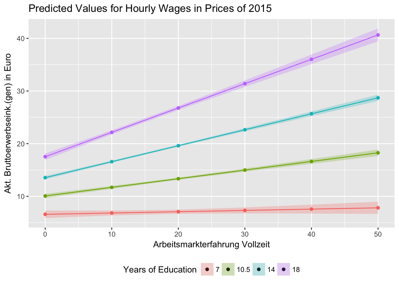
 # plot(dat, show.legend = F)+
 #       ggtitle("Predicted Values for Hourly Wages in Prices of 2015")+
 #       guides(fill=guide_legend(title="Years of Education"))
Coeff Plots
Marginal Effects of Work Experience
# Marginal Effect of Work Experience
      interplot(m = fit3.4 ,var1 = "erf", var2 = "pgbilzeit", hist = T)  +
            xlab("Education (in years)") +
            ylab("Estimated Coefficient for\n Work Experience") +
            ggtitle("Estimated Coefficient of Work Experience conditional on Education") +
            theme(plot.title = element_text(face="bold")) +
            geom_hline(yintercept = 0, linetype = "dashed")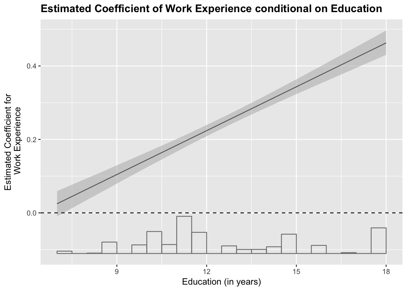
Marginal Effects of Education
# Marginal Effects of Education
      interplot(m=fit3.4, var1 = "pgbilzeit", var2="erf", point = F, hist = T) +
      theme(axis.text.x  = element_text(angle=45)) +
      xlab("Education (in years)") +
      ylab("Estimated Coefficient for\n Education") +
      ggtitle("Estimated Coefficient of Education \n on Hourly Wage conditional on Work Experience") +
      theme(plot.title = element_text(face="bold")) +
      # Add a horizontal line at y = 0
      geom_hline(yintercept = 0, linetype = "dashed")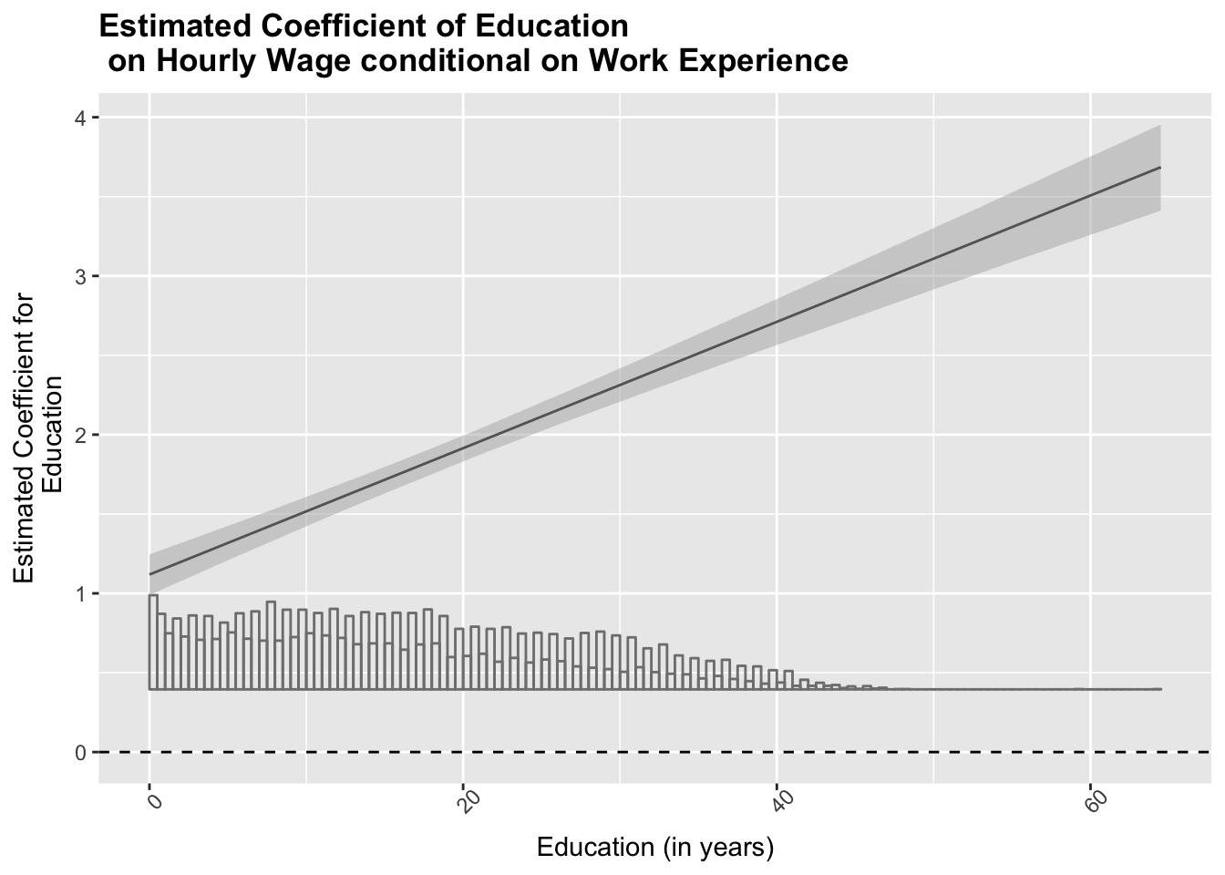
3.5 Nominal Variable
Include a nominal (e. g. company size: pgallbet) variable with more than two categories as predictors using a dummy set.
Stata
use "_data/ex_mydf.dta", clear

recode pgallbet (5 = 0)         // selbstst. keine Angest. als Referenz
reg hwageb i.frau##c.pgbilzeit c.pgbilzeit##c.erf ost i.pgallbet if asample==1 & syear==2015 [pw=phrf]

* OR
cap drop d_allbet
tab pgallbet, gen(d_allbet_)
reg hwageb i.frau##c.pgbilzeit c.pgbilzeit##c.erf ost d_allbet_2 - d_allbet_5 if asample==1 & syear==2015 [pw=phrf]
. use "_data/ex_mydf.dta", clear
(PGEN: Feb 12, 2017 13:00:53-1 DBV32L)

.
. recode pgallbet (5 = 0)                 // selbstst. keine Angest. als Refere
> nz
(pgallbet: 12302 changes made)

. reg hwageb i.frau##c.pgbilzeit c.pgbilzeit##c.erf ost i.pgallbet if asample==
> 1 & syear==2015 [pw=phrf]
(sum of wgt is   3.3642e+07)
note: pgbilzeit omitted because of collinearity

Linear regression                               Number of obs     =     14,099
                                                F(10, 14088)      =     228.22
                                                Prob > F          =     0.0000
                                                R-squared         =     0.2607
                                                Root MSE          =     9.8565

------------------------------------------------------------------------------
             |               Robust
      hwageb |      Coef.   Std. Err.      t    P>|t|     [95% Conf. Interval]
-------------+----------------------------------------------------------------
        frau |
   weiblich  |   .2678541    1.30856     0.20   0.838    -2.297098    2.832806
   pgbilzeit |   1.017978   .1221287     8.34   0.000     .7785891    1.257366
             |
        frau#|
 c.pgbilzeit |
   weiblich  |  -.2239346    .111358    -2.01   0.044    -.4422109   -.0056583
             |
   pgbilzeit |          0  (omitted)
         erf |  -.2735736   .0642253    -4.26   0.000    -.3994637   -.1476836
             |
 c.pgbilzeit#|
       c.erf |   .0405612   .0055719     7.28   0.000     .0296395    .0514828
             |
         ost |  -4.182231   .2730743   -15.32   0.000    -4.717493   -3.646969
             |
    pgallbet |
  [1] LT 20  |   .3324384   1.046256     0.32   0.751    -1.718361    2.383238
[2] GE 20..  |   1.250602   1.001918     1.25   0.212      -.71329    3.214494
[3] GE 20..  |    2.68006   1.016573     2.64   0.008     .6874428    4.672677
[4] GE 2000  |   4.739694   1.023765     4.63   0.000     2.732978    6.746409
             |
       _cons |  -.7349428   1.790305    -0.41   0.681    -4.244177    2.774292
------------------------------------------------------------------------------

.
. * OR
. cap drop d_allbet

. tab pgallbet, gen(d_allbet_)

     Grobkategorien Unternehmensgroesse |      Freq.     Percent        Cum.
----------------------------------------+-----------------------------------
                                      0 |     12,302        3.68        3.68
                              [1] LT 20 |     89,734       26.82       30.49
                       [2] GE 20 LT 200 |     89,910       26.87       57.36
                     [3] GE 200 LT 2000 |     68,415       20.45       77.81
                            [4] GE 2000 |     74,246       22.19      100.00
----------------------------------------+-----------------------------------
                                  Total |    334,607      100.00

. reg hwageb i.frau##c.pgbilzeit c.pgbilzeit##c.erf ost d_allbet_2 - d_allbet_5
>  if asample==1 & syear==2015 [pw=phrf]
(sum of wgt is   3.3642e+07)
note: pgbilzeit omitted because of collinearity

Linear regression                               Number of obs     =     14,099
                                                F(10, 14088)      =     228.22
                                                Prob > F          =     0.0000
                                                R-squared         =     0.2607
                                                Root MSE          =     9.8565

------------------------------------------------------------------------------
             |               Robust
      hwageb |      Coef.   Std. Err.      t    P>|t|     [95% Conf. Interval]
-------------+----------------------------------------------------------------
        frau |
   weiblich  |   .2678541    1.30856     0.20   0.838    -2.297098    2.832806
   pgbilzeit |   1.017978   .1221287     8.34   0.000     .7785891    1.257366
             |
        frau#|
 c.pgbilzeit |
   weiblich  |  -.2239346    .111358    -2.01   0.044    -.4422109   -.0056583
             |
   pgbilzeit |          0  (omitted)
         erf |  -.2735736   .0642253    -4.26   0.000    -.3994637   -.1476836
             |
 c.pgbilzeit#|
       c.erf |   .0405612   .0055719     7.28   0.000     .0296395    .0514828
             |
         ost |  -4.182231   .2730743   -15.32   0.000    -4.717493   -3.646969
  d_allbet_2 |   .3324384   1.046256     0.32   0.751    -1.718361    2.383238
  d_allbet_3 |   1.250602   1.001918     1.25   0.212      -.71329    3.214494
  d_allbet_4 |    2.68006   1.016573     2.64   0.008     .6874428    4.672677
  d_allbet_5 |   4.739694   1.023765     4.63   0.000     2.732978    6.746409
       _cons |  -.7349428   1.790305    -0.41   0.681    -4.244177    2.774292
------------------------------------------------------------------------------
R
if(!file.exists("out/fit3.5.rds")) {
      fit3.5 <- asample15 %>%
            lm(hwageb ~ pgbilzeit*frau + pgbilzeit*erf + ost + factor(pgallbet),
               data = ., weights = phrf)
      saveRDS(fit3.5, "out/fit3.5.rds")
} else {
      fit3.5 <- readRDS("out/fit3.5.rds")
}

tidy(fit3.5, conf.int = T)glance(fit3.5)3.6 Partial Effect Size
Drop the interactions and the dummy set. Include duration of unemployment pgexpue as additional predictor. What has the largest effect, years of education pgbilzeit, labor force experience erf or duration of unemployment pgexpue.
Years of education have the largest partial effect
standardization:
- if you wish to compare the partial effect sizes of the coefficients on your model, you need to standardize on both sides of the equations, the coefficients are then called beta- coefficients.
interpretation:
- beta- coefficients or standardized coefficients represent the change of y in terms of its standard deviation when x changes by 1 standard deviation. This way you can compare effect sizes of coefficients with different unit sizes.
Stata
use "_data/ex_mydf.dta", clear

reg hwageb pgbilzeit erf pgexpue frau ost if asample==1 & syear==2015 [pw=phrf] , beta
. use "_data/ex_mydf.dta", clear
(PGEN: Feb 12, 2017 13:00:53-1 DBV32L)

.
. reg hwageb pgbilzeit erf pgexpue frau ost if asample==1 & syear==2015 [pw=phr
> f] , beta
(sum of wgt is   3.3886e+07)

Linear regression                               Number of obs     =     14,218
                                                F(5, 14212)       =     255.50
                                                Prob > F          =     0.0000
                                                R-squared         =     0.2317
                                                Root MSE          =     10.031

------------------------------------------------------------------------------
             |               Robust
      hwageb |      Coef.   Std. Err.      t    P>|t|                     Beta
-------------+----------------------------------------------------------------
   pgbilzeit |    1.57627   .0626022    25.18   0.000                 .3805281
         erf |   .2355817   .0109985    21.42   0.000                 .2377894
     pgexpue |  -.4648154   .0429282   -10.83   0.000                -.0829968
        frau |  -2.735238    .241015   -11.35   0.000                -.1192848
         ost |  -3.793662   .2770086   -13.70   0.000                -.1262607
       _cons |  -5.405136   .7871563    -6.87   0.000                        .
------------------------------------------------------------------------------
R
fit3.6 <- asample15 %>%
      lm(hwageb ~ pgbilzeit +  erf + pgexpue + frau + ost,
         data=., weights=phrf)

tidy(fit3.6, conf.int = T)glance(fit3.6)look at analysis of variance table of fitted model objects
anova(fit3.6)get beta coefficients for model with lm.beta package more info here
lm.fit3.6.beta <- lm.beta(fit3.6)
lm.fit3.6.beta # or coef(lm.fit3.6.beta)
##
## Call:
## lm(formula = hwageb ~ pgbilzeit + erf + pgexpue + frau + ost,
## data = ., weights = phrf)
##
## Standardized Coefficients::
## (Intercept) pgbilzeit erf pgexpue fraufemale osteast
## 0.000 0.366 0.215 -0.079 -0.114 -0.124Summary of model and beta’s (standardized)
summary(lm.fit3.6.beta)##
## Call:
## lm(formula = hwageb ~ pgbilzeit + erf + pgexpue + frau + ost,
## data = ., weights = phrf)
##
## Weighted Residuals:
## Min 1Q Median 3Q Max
## -2649 -150 -15 117 19910
##
## Coefficients:
## Estimate Standardized Std. Error t value Pr(>|t|)
## (Intercept) -5.40520 0.00000 0.47447 -11.4 <2e-16 ***
## pgbilzeit 1.57628 0.36631 0.03142 50.2 <2e-16 ***
## erf 0.23558 0.21523 0.00762 30.9 <2e-16 ***
## pgexpue -0.46481 -0.07930 0.04272 -10.9 <2e-16 ***
## fraufemale -2.73528 -0.11444 0.17300 -15.8 <2e-16 ***
## osteast -3.79364 -0.12432 0.22581 -16.8 <2e-16 ***
## ---
## Signif. codes: 0 '***' 0.001 '**' 0.01 '*' 0.05 '.' 0.1 ' ' 1
##
## Residual standard error: 490 on 14213 degrees of freedom
## (549 observations deleted due to missingness)
## Multiple R-squared: 0.232, Adjusted R-squared: 0.231
## F-statistic: 857 on 5 and 14213 DF, p-value: <2e-163.7 Quadratic Effect
Specify a quadratic effect for labor force participation. Interpret the result using a marginal effects plot.
The marginsplot shows that the effect of work experience is quadratic, meaning that work experience has a stronger positive effect on hourly wage in the beginnign of a career, while the effect becomes smaller at the end of the career. It is also important to note that the confidence intervals are getting larger from 30 years of work experience onwards.
Stata
Model
use "_data/ex_mydf.dta", clear

reg hwageb pgbilzeit c.erf##c.erf frau ost if asample==1 & syear==2015 [pw=phrf]

qui: margins, at(erf=(0(10)65))
marginsplot
graph export "out/margins_3_7.eps", replace

reg hwageb pgbilzeit c.erf##c.erf frau ost if asample==1 & syear==2015 [pw=phrf]

qui: margins, at(erf=(0(10)50) pgbilzeit=(7, 10.5, 14, 18) frau=(1 0))
marginsplot
graph export "out/margins_3_7_2.eps", replace
. use "_data/ex_mydf.dta", clear
(PGEN: Feb 12, 2017 13:00:53-1 DBV32L)

.
. reg hwageb pgbilzeit c.erf##c.erf frau ost if asample==1 & syear==2015 [pw=ph
> rf]
(sum of wgt is   3.3886e+07)

Linear regression                               Number of obs     =     14,218
                                                F(5, 14212)       =     223.24
                                                Prob > F          =     0.0000
                                                R-squared         =     0.2354
                                                Root MSE          =     10.007

------------------------------------------------------------------------------
             |               Robust
      hwageb |      Coef.   Std. Err.      t    P>|t|     [95% Conf. Interval]
-------------+----------------------------------------------------------------
   pgbilzeit |   1.616197    .061299    26.37   0.000     1.496043    1.736351
         erf |    .585291   .0352085    16.62   0.000     .5162778    .6543042
             |
 c.erf#c.erf |  -.0088073    .000908    -9.70   0.000    -.0105872   -.0070275
             |
        frau |  -2.914366   .2435542   -11.97   0.000    -3.391764   -2.436968
         ost |  -4.191624   .2685655   -15.61   0.000    -4.718047     -3.6652
       _cons |  -8.353138   .7982404   -10.46   0.000    -9.917793   -6.788482
------------------------------------------------------------------------------

.
. qui: margins, at(erf=(0(10)65))

. marginsplot

  Variables that uniquely identify margins: erf

. graph export "out/margins_3_7.eps", replace
(file out/margins_3_7.eps written in EPS format)

.
. reg hwageb pgbilzeit c.erf##c.erf frau ost if asample==1 & syear==2015 [pw=ph
> rf]
(sum of wgt is   3.3886e+07)

Linear regression                               Number of obs     =     14,218
                                                F(5, 14212)       =     223.24
                                                Prob > F          =     0.0000
                                                R-squared         =     0.2354
                                                Root MSE          =     10.007

------------------------------------------------------------------------------
             |               Robust
      hwageb |      Coef.   Std. Err.      t    P>|t|     [95% Conf. Interval]
-------------+----------------------------------------------------------------
   pgbilzeit |   1.616197    .061299    26.37   0.000     1.496043    1.736351
         erf |    .585291   .0352085    16.62   0.000     .5162778    .6543042
             |
 c.erf#c.erf |  -.0088073    .000908    -9.70   0.000    -.0105872   -.0070275
             |
        frau |  -2.914366   .2435542   -11.97   0.000    -3.391764   -2.436968
         ost |  -4.191624   .2685655   -15.61   0.000    -4.718047     -3.6652
       _cons |  -8.353138   .7982404   -10.46   0.000    -9.917793   -6.788482
------------------------------------------------------------------------------

.
. qui: margins, at(erf=(0(10)50) pgbilzeit=(7, 10.5, 14, 18) frau=(1 0))

. marginsplot

  Variables that uniquely identify margins: erf pgbilzeit frau

. graph export "out/margins_3_7_2.eps", replace
(file out/margins_3_7_2.eps written in EPS format)

.
Plot
Marginsplot Work Experience Squared
knitr::include_graphics("out/margins_3_7.png")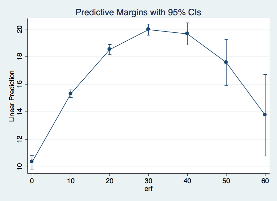
Margins Plot Work Experience Conditional on Education and Gender
knitr::include_graphics("out/margins_3_7_2.png")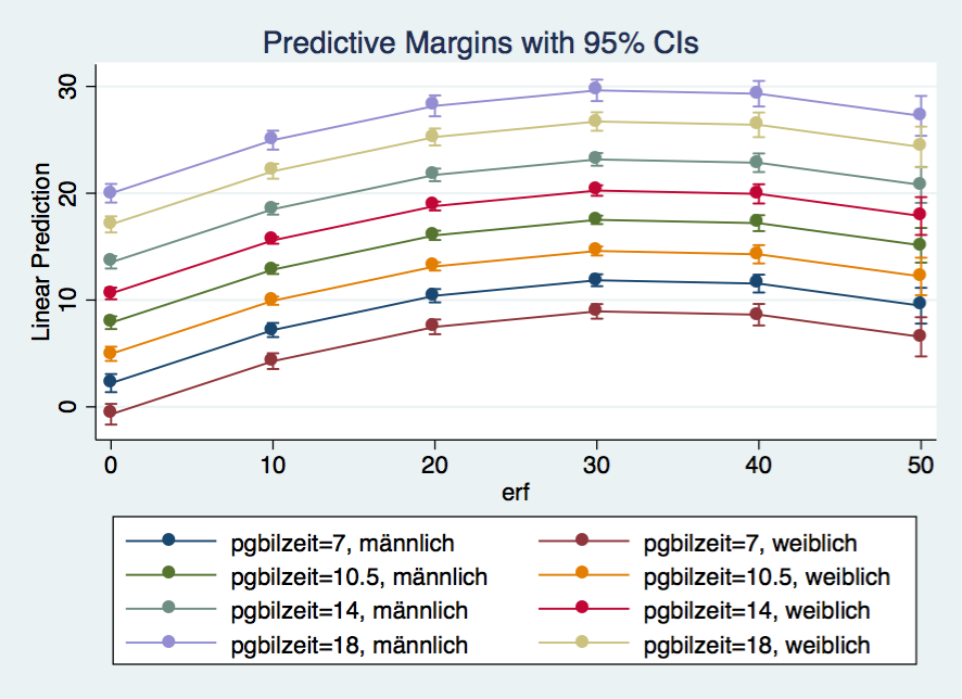
R
Models
Fit 3.7
fit3.7 <- asample15 %>%
                  lm(hwageb ~ pgbilzeit + erf + I(erf^2) + frau + ost,
                     data=., weights=phrf)

tidy(fit3.7, conf.int = T)glance(fit3.7)Plots
Margins Plot Work Experience
 # for polynomial data
 dat <- ggpredict(fit3.7, terms = c("erf [0,10, 20, 30, 40, 50]"))

 ggplot(dat, aes(x, predicted)) +
       stat_smooth(se = FALSE) +
       geom_ribbon(aes(ymin = conf.low, ymax = conf.high), alpha = .15) +
       labs(x = get_x_title(dat), y = get_y_title(dat))
## `geom_smooth()` using method = 'loess'## Warning in simpleLoess(y, x, w, span, degree = degree, parametric =
## parametric, : Chernobyl! trL>n 6
## Warning in simpleLoess(y, x, w, span, degree = degree, parametric =
## parametric, : Chernobyl! trL>n 6## Warning in sqrt(sum.squares/one.delta): NaNs wurden erzeugt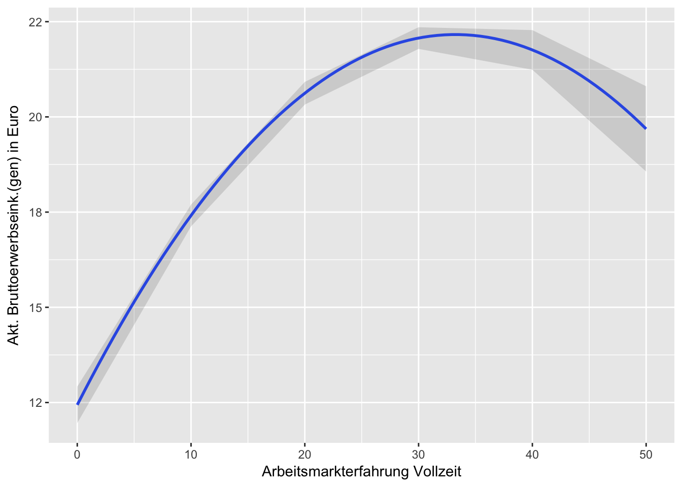
 # quick alternative
 # plot(dat)
Margins Plot Work Experience Conditional on Education and Gender
dat <- ggpredict(fit3.7, terms = c("erf [0,10,20,30,40,50]", "pgbilzeit [7,10.5,14,18]", "frau"))

ggplot(dat, aes(x, predicted, color = group, fill = group, linetype = facet)) +
       geom_point()+
       geom_line()+
      geom_ribbon(ggplot2::aes_string(ymin = "conf.low",
                ymax = "conf.high", color = NULL), alpha = 0.25)+
       labs(x = get_x_title(dat), y = get_y_title(dat))+
       ggtitle("Predicted Values for Hourly Wage in Prices of 2015")+
       theme(legend.position="bottom")+
       guides(fill = guide_legend(title="Years of Work Experience"),
              linetype = guide_legend(title = "Gender"),
              color = F)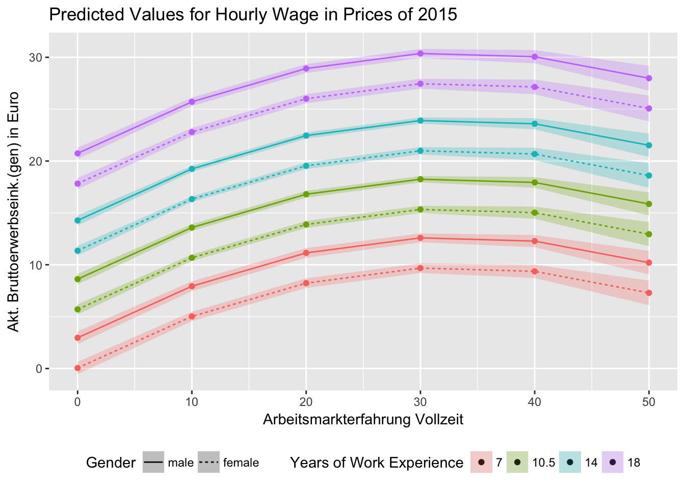
3.8 Log Transformation
Now, use log-transformed income lnwage as dependent variable. Interpret the effect of years of education pgbilzeit on income. Present your result in a table using estout or esttab.
Stata
use "_data/ex_mydf.dta", clear

reg lnwage pgbilzeit c.erf##c.erf frau ost if asample==1 & syear==2015 [pw=phrf]
estimates store est1

* esttab
esttab

* estout
estout

* outreg
outreg2 est1 using "out/table3.8.xls", excel replace label alpha(0.001, 0.01, 0.05) bdec(3) eform stats(coef se)
. use "_data/ex_mydf.dta", clear
(PGEN: Feb 12, 2017 13:00:53-1 DBV32L)

.
. reg lnwage pgbilzeit c.erf##c.erf frau ost if asample==1 & syear==2015 [pw=ph
> rf]
(sum of wgt is   3.3697e+07)

Linear regression                               Number of obs     =     14,150
                                                F(5, 14144)       =     391.34
                                                Prob > F          =     0.0000
                                                R-squared         =     0.2969
                                                Root MSE          =     .48037

------------------------------------------------------------------------------
             |               Robust
      lnwage |      Coef.   Std. Err.      t    P>|t|     [95% Conf. Interval]
-------------+----------------------------------------------------------------
   pgbilzeit |   .0856499   .0026784    31.98   0.000     .0803999    .0908999
         erf |   .0381035   .0022446    16.98   0.000     .0337039    .0425032
             |
 c.erf#c.erf |  -.0005924   .0000521   -11.36   0.000    -.0006946   -.0004902
             |
        frau |  -.1456176   .0137884   -10.56   0.000    -.1726446   -.1185906
         ost |  -.2642993   .0176628   -14.96   0.000    -.2989206   -.2296779
       _cons |   1.270545   .0429209    29.60   0.000     1.186414    1.354675
------------------------------------------------------------------------------

. estimates store est1

.
. * esttab
. esttab

----------------------------
                      (1)
                   lnwage
----------------------------
pgbilzeit          0.0856***
                  (31.98)

erf                0.0381***
                  (16.98)

c.erf#c.erf     -0.000592***
                 (-11.36)

frau               -0.146***
                 (-10.56)

ost                -0.264***
                 (-14.96)

_cons               1.271***
                  (29.60)
----------------------------
N                   14150
----------------------------
t statistics in parentheses
* p<0.05, ** p<0.01, *** p<0.001

.
. * estout
. estout

-------------------------
                     est1
                        b
-------------------------
pgbilzeit        .0856499
erf              .0381035
c.erf#c.erf     -.0005924
frau            -.1456176
ost             -.2642993
_cons            1.270545
-------------------------

.
. * outreg
. outreg2 est1 using "out/table3.8.xls", excel replace label alpha(0.001, 0.01,
>  0.05) bdec(3) eform stats(coef se)
out/table3.8.xls
dir : seeout
R
fit3.8 <- asample15 %>%
      lm(lnwage ~ pgbilzeit + erf + I(erf^2) + frau + ost,
         data=., weights=phrf)

tidy(fit3.8)glance(fit3.8)stargazer(fit3.8, type = "html",
title ="Regression Results",
dep.var.labels= c("Hourly Wages in Prices of 2015"),
out = "out/model_3.8.txt")| Dependent variable: | |
| Hourly Wages in Prices of 2015 | |
| pgbilzeit | 0.086*** |
| (0.001) | |
| erf | 0.038*** |
| (0.001) | |
| I(erf2) | -0.001*** |
| (0.00003) | |
| frau | -0.150*** |
| (0.008) | |
| ost | -0.270*** |
| (0.011) | |
| Constant | 1.300*** |
| (0.023) | |
| Observations | 14,232 |
| R2 | 0.300 |
| Adjusted R2 | 0.300 |
| Residual Std. Error | 23.000 (df = 14147) |
| F Statistic | 1,198.000*** (df = 5; 14147) |
| Note: | p<0.1; p<0.05; p<0.01 |