4.1 Cross-Level Interaction Model
Model Data
Stata
use "_data/ess50prep.dta", clear

xtmixed stfdem polintr nwsptot gndr##newest gndr##new || cntry: gndr, cov(unstructured)
estat icc
. use "_data/ess50prep.dta", clear

.
. xtmixed stfdem polintr nwsptot gndr##newest gndr##new || cntry: gndr, cov(uns
> tructured)

Performing EM optimization:

Performing gradient-based optimization:

Iteration 0:   log likelihood = -24309.031
Iteration 1:   log likelihood = -24309.028
Iteration 2:   log likelihood = -24309.028

Computing standard errors:

Mixed-effects ML regression                     Number of obs     =     10,963
Group variable: cntry                           Number of groups  =         22

                                                Obs per group:
                                                              min =         46
                                                              avg =      498.3
                                                              max =      1,544

                                                Wald chi2(7)      =     114.61
Log likelihood = -24309.028                     Prob > chi2       =     0.0000

------------------------------------------------------------------------------
      stfdem |      Coef.   Std. Err.      z    P>|z|     [95% Conf. Interval]
-------------+----------------------------------------------------------------
     polintr |  -.2399529    .025955    -9.24   0.000    -.2908237   -.1890821
     nwsptot |   .0058149   .0177282     0.33   0.743    -.0289317    .0405615
             |
        gndr |
     female  |  -.1657879   .0645948    -2.57   0.010    -.2923914   -.0391843
    1.newest |  -1.140559    .368079    -3.10   0.002    -1.861981   -.4191378
             |
 gndr#newest |
   female#1  |   .1723873   .1302671     1.32   0.186    -.0829316    .4277062
             |
       1.new |  -.2253065   .4165704    -0.54   0.589    -1.041769    .5911564
             |
    gndr#new |
   female#1  |   .0888319   .1532403     0.58   0.562    -.2115135    .3891773
             |
       _cons |   6.366919   .1856832    34.29   0.000     6.002986    6.730851
------------------------------------------------------------------------------

------------------------------------------------------------------------------
  Random-effects Parameters  |   Estimate   Std. Err.     [95% Conf. Interval]
-----------------------------+------------------------------------------------
cntry: Unstructured          |
                    sd(gndr) |   .1258337    .073777      .0398779    .3970644
                   sd(_cons) |   .6765851   .1251705      .4708117     .972294
            corr(gndr,_cons) |  -.3937098   .3608483     -.8491707    .3976095
-----------------------------+------------------------------------------------
                sd(Residual) |   2.213484   .0149805      2.184316    2.243041
------------------------------------------------------------------------------
LR test vs. linear model: chi2(3) = 690.66                Prob > chi2 = 0.0000

Note: LR test is conservative and provided only for reference.

. estat icc

Conditional intraclass correlation

------------------------------------------------------------------------------
                       Level |        ICC   Std. Err.     [95% Conf. Interval]
-----------------------------+------------------------------------------------
                       cntry |   .0854478   .0289368      .0432608    .1618164
------------------------------------------------------------------------------
Note: ICC is conditional on zero values of random-effects covariates.
R
multi4 <- lmer(stfdem ~ polintr + nwsptot + (gndr * new) + (gndr * newest) + (1 + gndr |cntry), data = ess, REML = FALSE)tidy(multi4)glance(multi4)icc(multi4)##
## Linear mixed model
## Family: gaussian (identity)
## Formula: stfdem ~ polintr + nwsptot + (gndr * new) + (gndr * newest) + (1 + gndr | cntry)
##
## ICC (cntry): 0.0854464.2 Fixed Effects Plots
Stata
not (yet) available
R
Fixed effects
p-values approximated by Wald-Statistics with p.kr = FALSE -> reduces computing time signficantly
sjp.lmer(multi4, type = "fe", p.kr = FALSE)## Computing p-values via Wald-statistics approximation (treating t as Wald z).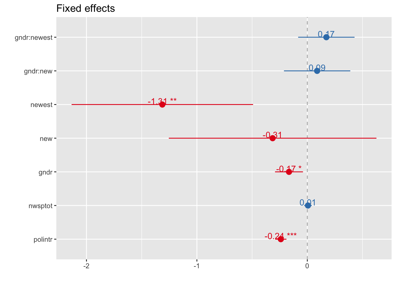
Standardized Fixed effects
sjp.lmer(multi4, type = "fe.std", p.kr = FALSE)## Computing p-values via Wald-statistics approximation (treating t as Wald z).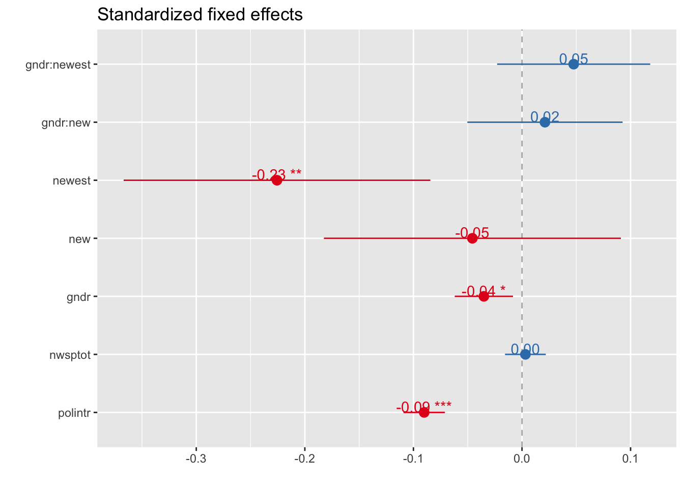
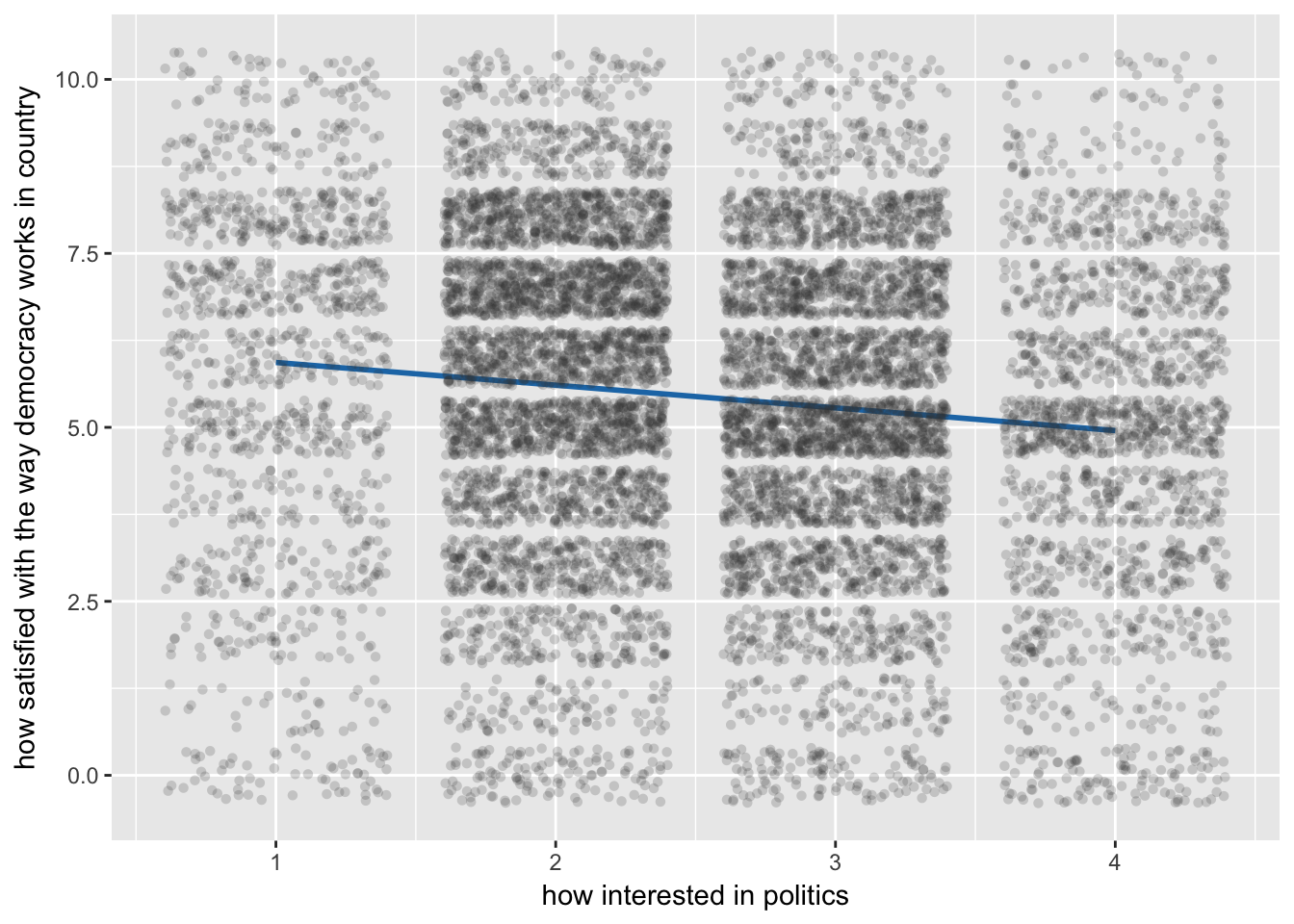
Slopes of fixed effects
sjp.lmer(multi4, type = "fe.slope", vars = c("newest", "polintr"))## `sjp.lmer()` will become deprecated in the future. Please use `plot_model()` instead.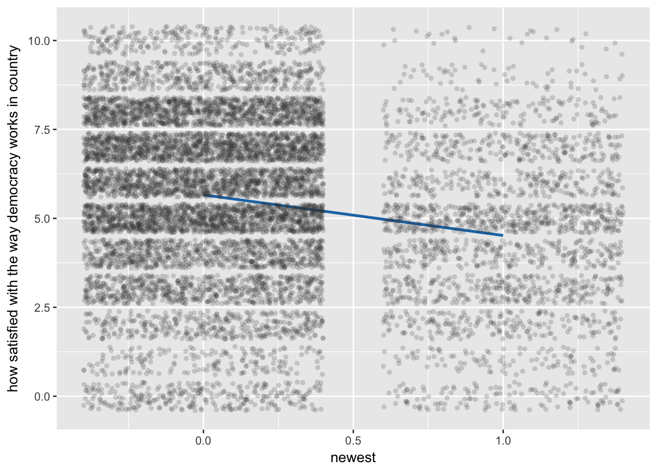
## Don't know how to automatically pick scale for object of type labelled. Defaulting to continuous.