3. Random Coefficient Model
3.1 Without Gender Variable
Stata
use "_data/ess50prep.dta", clear

xtmixed stfdem polintr nwsptot || cntry: polintr nwsptot, cov(unstructured)
estat icc
. use "_data/ess50prep.dta", clear

.
. xtmixed stfdem polintr nwsptot || cntry: polintr nwsptot, cov(unstructured)

Performing EM optimization:

Performing gradient-based optimization:

Iteration 0:   log likelihood = -24343.339
Iteration 1:   log likelihood =  -24342.86
Iteration 2:   log likelihood = -24342.858

Computing standard errors:
standard-error calculation failed

Mixed-effects ML regression                     Number of obs     =     10,977
Group variable: cntry                           Number of groups  =         22

                                                Obs per group:
                                                              min =         46
                                                              avg =      499.0
                                                              max =      1,544

                                                Wald chi2(2)      =      41.94
Log likelihood = -24342.858                     Prob > chi2       =     0.0000

------------------------------------------------------------------------------
      stfdem |      Coef.   Std. Err.      z    P>|z|     [95% Conf. Interval]
-------------+----------------------------------------------------------------
     polintr |  -.2418052   .0385597    -6.27   0.000    -.3173807   -.1662297
     nwsptot |   .0075553   .0177033     0.43   0.670    -.0271425    .0422531
       _cons |    6.06071   .2056077    29.48   0.000     5.657726    6.463694
------------------------------------------------------------------------------

------------------------------------------------------------------------------
  Random-effects Parameters  |   Estimate   Std. Err.     [95% Conf. Interval]
-----------------------------+------------------------------------------------
cntry: Unstructured          |
                 sd(polintr) |   .1269699          .             .           .
                 sd(nwsptot) |   .0058373          .             .           .
                   sd(_cons) |   .8789842          .             .           .
       corr(polintr,nwsptot) |   .6191228          .             .           .
         corr(polintr,_cons) |  -.5714132          .             .           .
         corr(nwsptot,_cons) |  -.9982364          .             .           .
-----------------------------+------------------------------------------------
                sd(Residual) |   2.212509          .             .           .
------------------------------------------------------------------------------
LR test vs. linear model: chi2(6) = 1099.26               Prob > chi2 = 0.0000

Note: LR test is conservative and provided only for reference.

. estat icc

Conditional intraclass correlation

------------------------------------------------------------------------------
                       Level |        ICC   Std. Err.     [95% Conf. Interval]
-----------------------------+------------------------------------------------
                       cntry |    .136316          0       .136316     .136316
------------------------------------------------------------------------------
Note: ICC is conditional on zero values of random-effects covariates.
R
First: Save Model (like Stata’s est store)
multi3 <- lmer(stfdem ~ polintr + nwsptot + (1 + polintr + nwsptot |cntry), data = ess, REML = FALSE)1 + is not necessarily needed because random coefficient models imply that the intercept is also random
Then: Inspect model
tidy(multi3)glance(multi3)icc(multi3)##
## Linear mixed model
## Family: gaussian (identity)
## Formula: stfdem ~ (1 + polintr + nwsptot | cntry)
##
## ICC (cntry): 0.1849943.2 With gender variable
Stata
set maxiter 20
use "_data/ess50prep.dta", clear

xtmixed stfdem || cntry: polintr nwsptot gndr, cov(unstructured)
. set maxiter 20

. use "_data/ess50prep.dta", clear

.
. xtmixed stfdem || cntry: polintr nwsptot gndr, cov(unstructured)

Performing EM optimization:

Performing gradient-based optimization:

Iteration 0:   log likelihood = -24320.636
Iteration 1:   log likelihood = -24320.137
Iteration 2:   log likelihood = -24320.135  (not concave)
Iteration 3:   log likelihood = -24320.135  (not concave)
Iteration 4:   log likelihood = -24320.135  (not concave)
Iteration 5:   log likelihood = -24320.135  (not concave)
Iteration 6:   log likelihood = -24320.135  (not concave)
Iteration 7:   log likelihood = -24320.135  (not concave)
Iteration 8:   log likelihood = -24320.135  (not concave)
Iteration 9:   log likelihood = -24320.135  (not concave)
Iteration 10:  log likelihood = -24320.135  (not concave)
Iteration 11:  log likelihood = -24320.135  (not concave)
Iteration 12:  log likelihood = -24320.135  (not concave)
Iteration 13:  log likelihood = -24320.135  (not concave)
Iteration 14:  log likelihood = -24320.135  (not concave)
Iteration 15:  log likelihood = -24320.135  (not concave)
Iteration 16:  log likelihood = -24320.135  (not concave)
Iteration 17:  log likelihood = -24320.135  (not concave)
Iteration 18:  log likelihood = -24320.135  (not concave)
Iteration 19:  log likelihood = -24320.135  (not concave)
Iteration 20:  log likelihood = -24320.135  (not concave)
convergence not achieved

Computing standard errors:
standard-error calculation failed

Mixed-effects ML regression                     Number of obs     =     10,963
Group variable: cntry                           Number of groups  =         22

                                                Obs per group:
                                                              min =         46
                                                              avg =      498.3
                                                              max =      1,544

                                                Wald chi2(0)      =          .
Log likelihood = -24320.135                     Prob > chi2       =          .

------------------------------------------------------------------------------
      stfdem |      Coef.   Std. Err.      z    P>|z|     [95% Conf. Interval]
-------------+----------------------------------------------------------------
       _cons |   5.413475     .15805    34.25   0.000     5.103703    5.723247
------------------------------------------------------------------------------

------------------------------------------------------------------------------
  Random-effects Parameters  |   Estimate   Std. Err.     [95% Conf. Interval]
-----------------------------+------------------------------------------------
cntry: Unstructured          |
                 sd(polintr) |   .2580515          .             .           .
                 sd(nwsptot) |   .0113277          .             .           .
                    sd(gndr) |   .1666332          .             .           .
                   sd(_cons) |   1.186181          .             .           .
       corr(polintr,nwsptot) |  -.0364619          .             .           .
          corr(polintr,gndr) |   .6040483          .             .           .
         corr(polintr,_cons) |  -.7291646          .             .           .
          corr(nwsptot,gndr) |  -.4848374          .             .           .
         corr(nwsptot,_cons) |  -.3091991          .             .           .
            corr(gndr,_cons) |  -.6714956          .             .           .
-----------------------------+------------------------------------------------
                sd(Residual) |   2.211121          .             .           .
------------------------------------------------------------------------------
LR test vs. linear model: chi2(10) = 1252.33              Prob > chi2 = 0.0000

Note: LR test is conservative and provided only for reference.
Warning: convergence not achieved; estimates are based on iterated EM
R
First: Save Model (like Stata’s est store)
multi3 <- lmer(stfdem ~ (1 + polintr + nwsptot + gndr |cntry), data = ess, REML = FALSE)Then: Inspect model
tidy(multi3)glance(multi3)icc(multi3)##
## Linear mixed model
## Family: gaussian (identity)
## Formula: stfdem ~ (1 + polintr + nwsptot + gndr | cntry)
##
## ICC (cntry): 0.2234893.3 Plotting data
Stata
not (yet) available
R
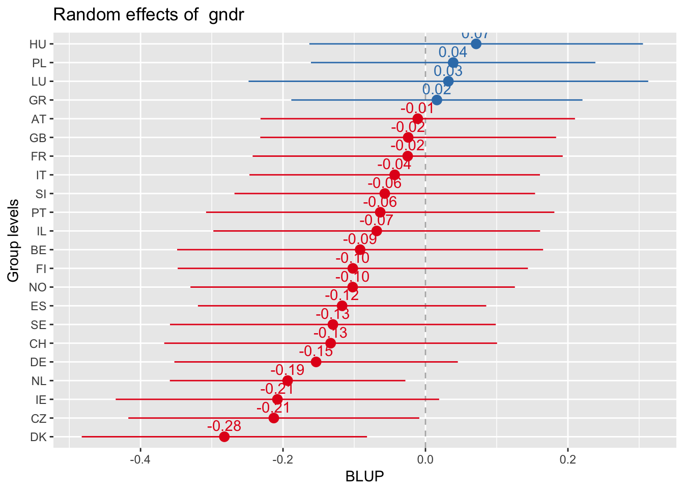
Random effect plots
Sorted alphabetically
sjp.lmer(multi3, y.offset = .6)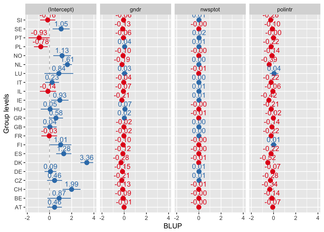
Everything sorted by values of intercept
sjp.lmer(multi3, sort.est = "(Intercept)", y.offset = .6)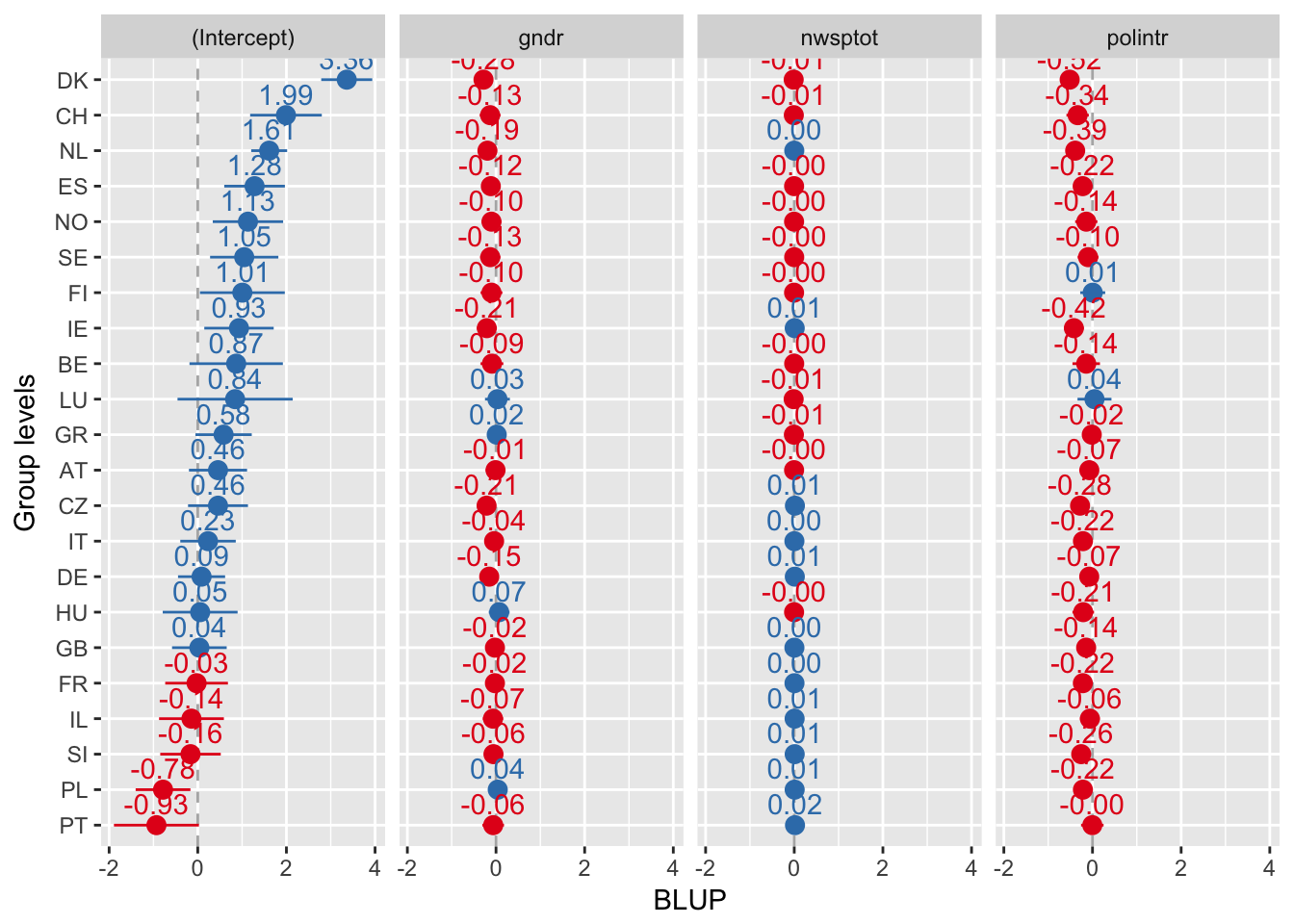
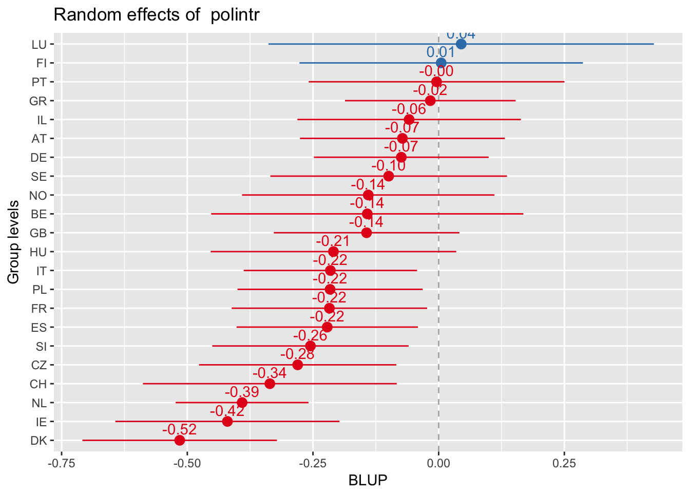
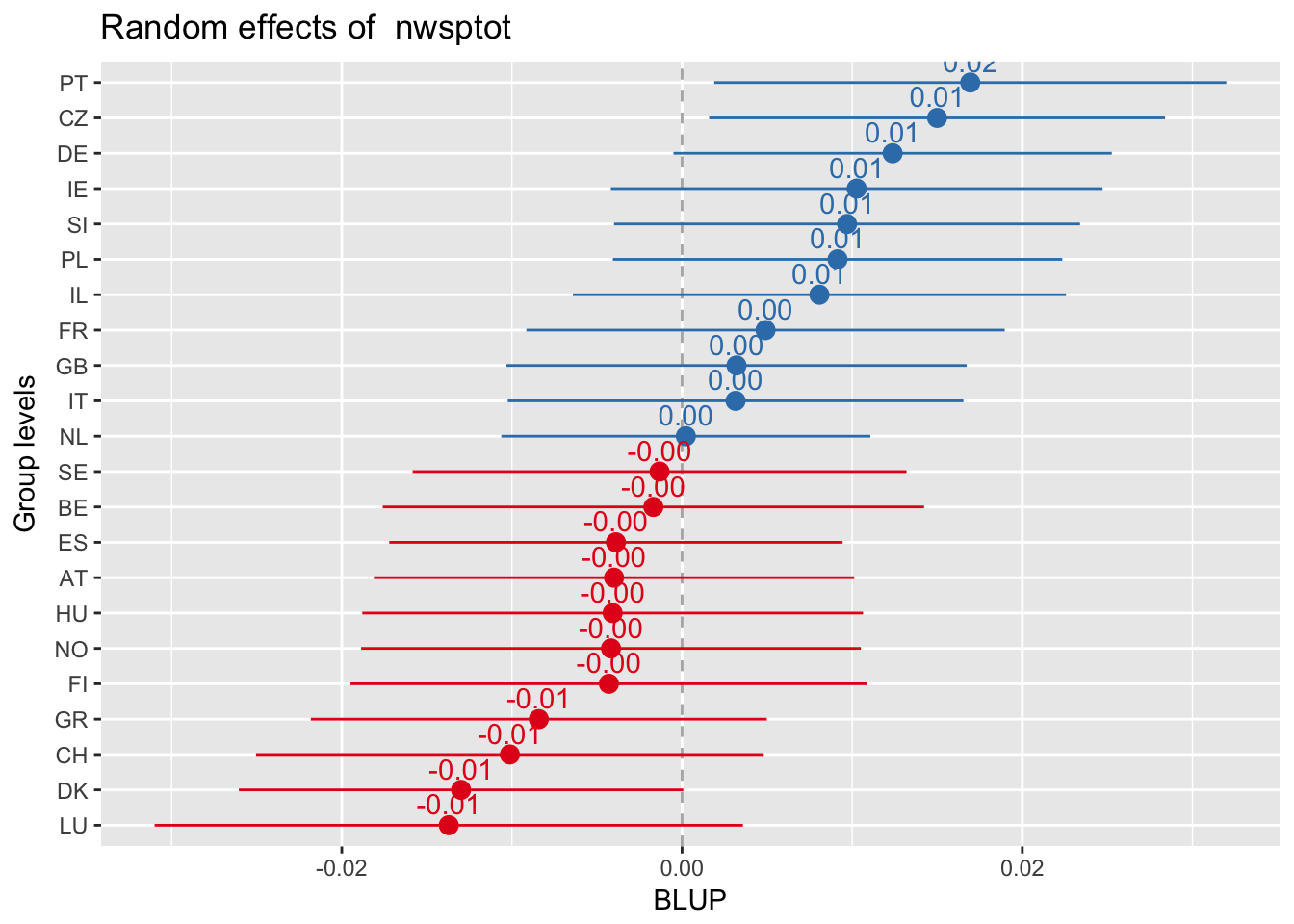
Every plot sorted by its own values
sjp.lmer(multi3, sort.est = "sort.all", y.offset = .6, facet.grid = FALSE)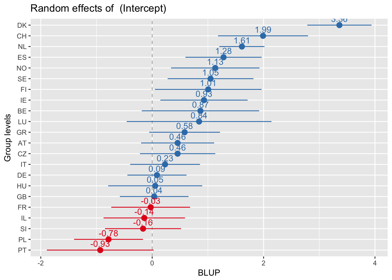
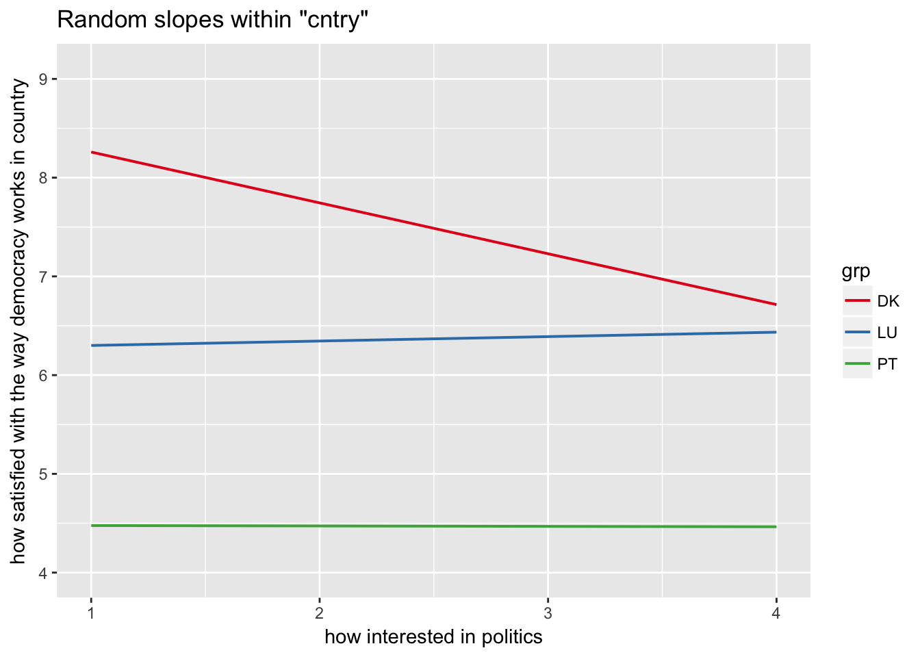
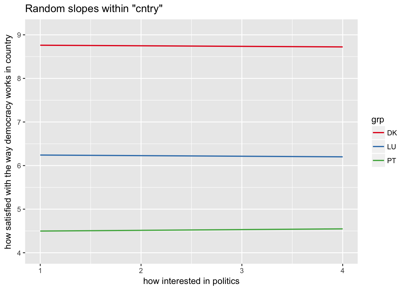
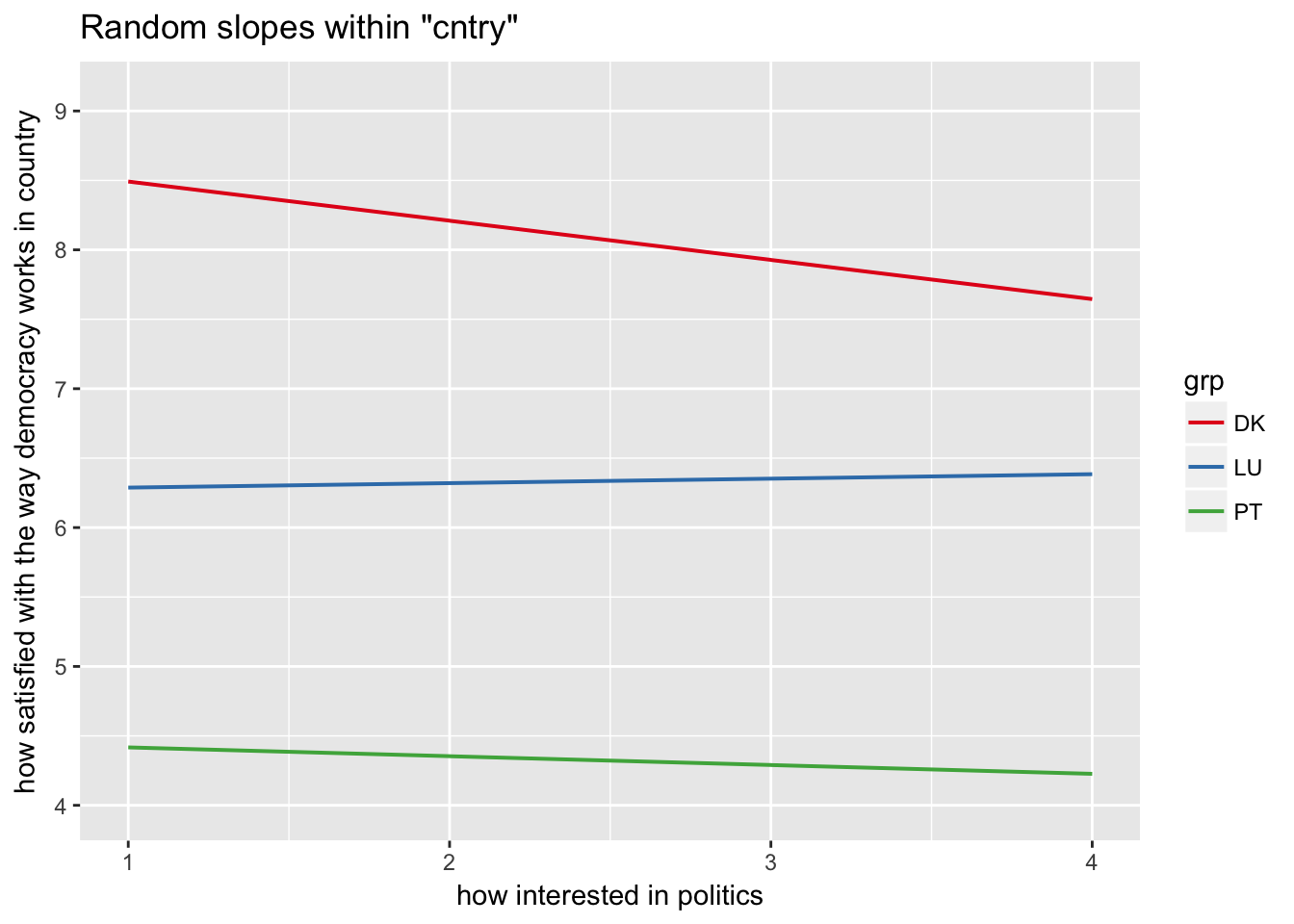
Random slopes plots
Random slopes depending on random intercepts
sjp.lmer(multi3, type = "rs.ri", vars = "polintr", show.legend = TRUE)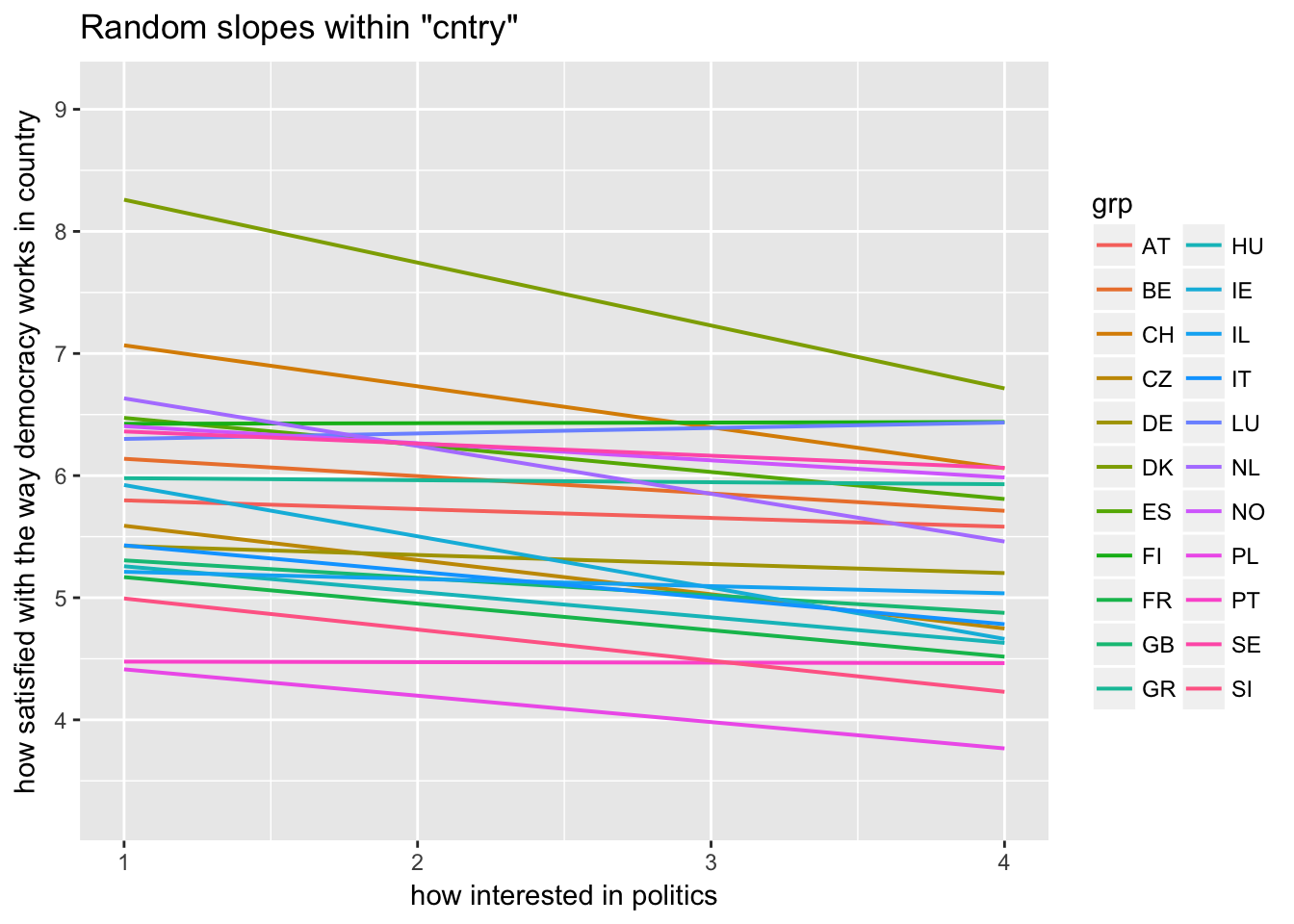
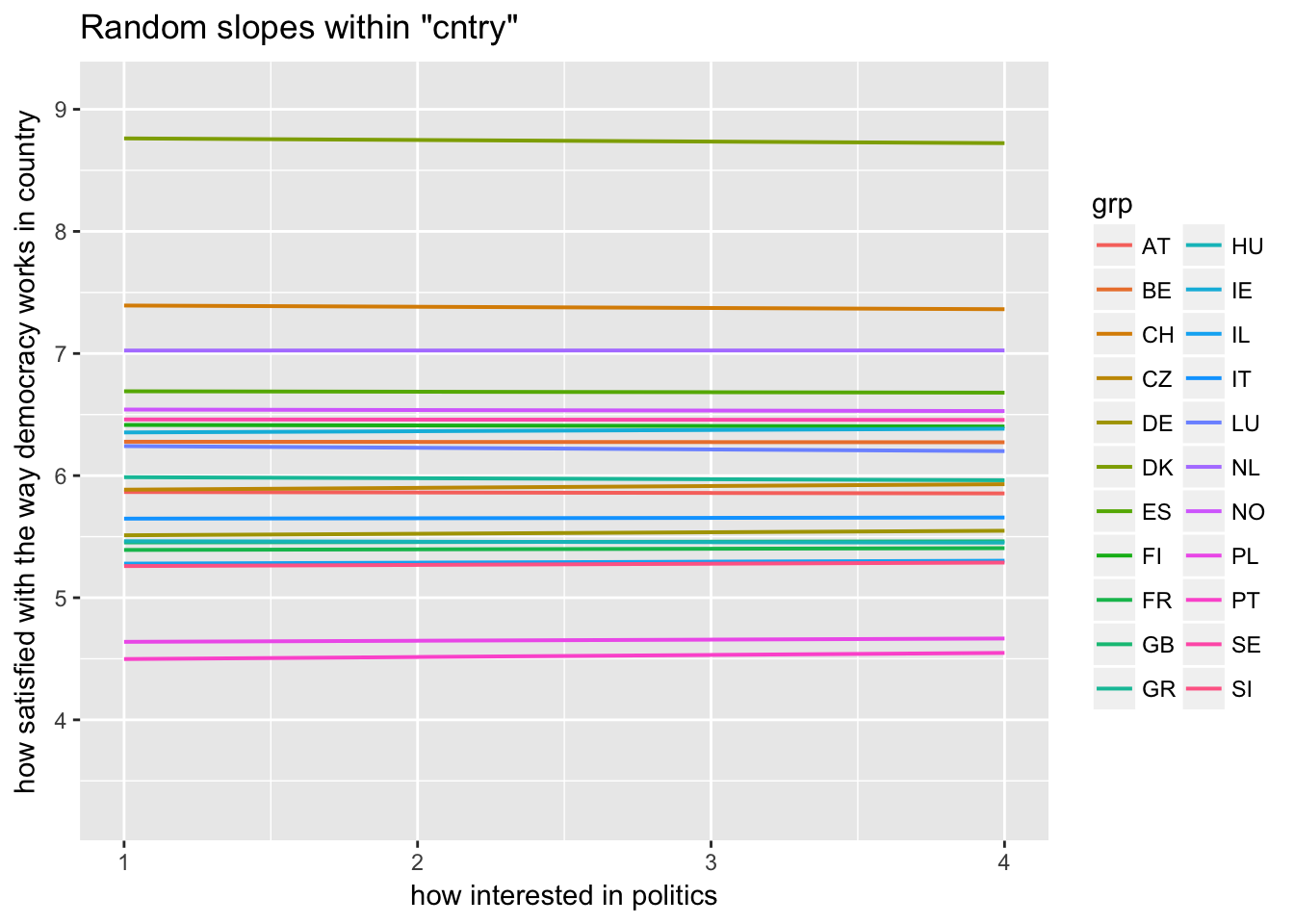
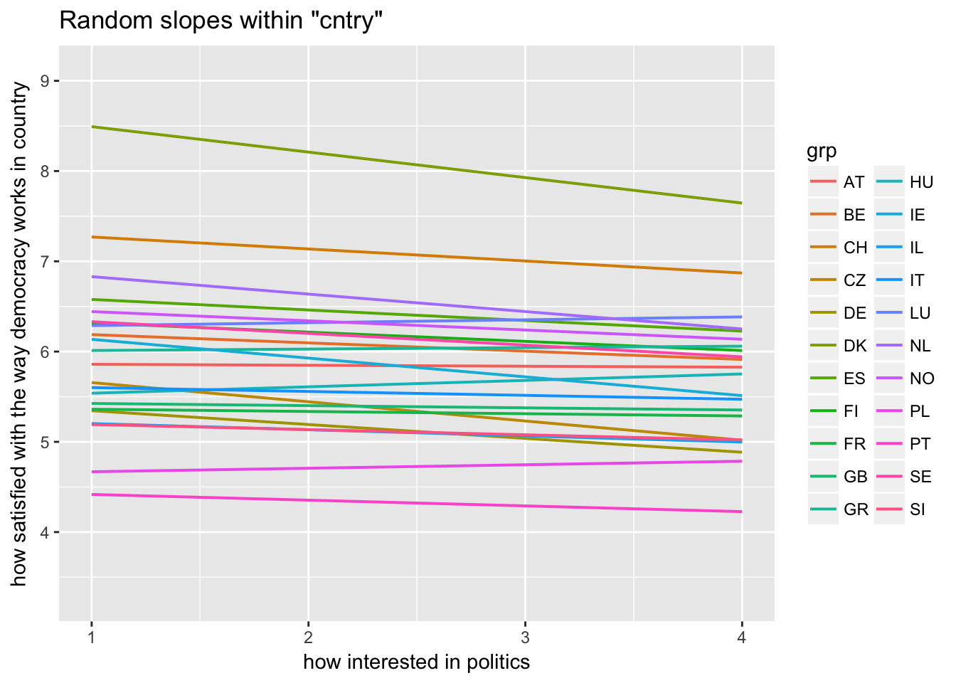
Random slopes depending on random intercepts highlighting Denmark, Portugal, Luxemburg
sjp.lmer(multi3, type = "rs.ri", vars = "polintr", sample.n = c(6, 16, 20), show.legend = TRUE)