Exercise 2
Questions
2.1 Estimate a Linear Regression with SOEP Data using hourly wage
hwagebas dependent variable for the year 2015. Include years of schoolingpgbilzeitand work experienceerfas predictor variables and genderfrauand regionostas additional controls.2.2 Interpret the coefficients and the value of R²
2.3 Is the relationship between work experience and wage linear?
2.4 Specifiy the same regression model but use the natural logarithm
lnwageas dependent variable instead.2.5 How large is the gender pay gap?
Data Prep
Stata
use "_data/ex_mydf.dta", clear

* Unplausible Beobachtungen identifizieren
********************************************************************************
      twoway (scatter hwageb pgtatzeit, msymbol(point) jitter(2))

* Visualize Income
********************************************************************************
      histogram hwageb if asample==1, bin(25)
    sum hwageb if asample==1, d
    twoway (scatter hwageb pgtatzeit, msymbol(point) jitter(2)) if asample==1
. use "_data/ex_mydf.dta", clear
(PGEN: Feb 12, 2017 13:00:53-1 DBV32L)

.
. * Unplausible Beobachtungen identifizieren
. *****************************************************************************
> ***
.       twoway (scatter hwageb pgtatzeit, msymbol(point) jitter(2))

.
. * Visualize Income
. *****************************************************************************
> ***
.       histogram hwageb if asample==1, bin(25)
(bin=25, start=0, width=30.855825)

.         sum hwageb if asample==1, d

             Hourly Brutto Income in 2015 Prices
-------------------------------------------------------------
      Percentiles      Smallest
 1%     2.169231              0
 5%     5.403614              0
10%     7.005816              0       Obs             305,838
25%     9.983869              0       Sum of Wgt.     305,838

50%     14.00146                      Mean           16.06223
                        Largest       Std. Dev.      11.46355
75%     19.18718        525.431
90%     26.40982       556.8619       Variance        131.413
95%     32.53085       559.2414       Skewness       8.248211
99%     54.21809       771.3956       Kurtosis       224.3553

.         twoway (scatter hwageb pgtatzeit, msymbol(point) jitter(2)) if asampl
> e==1

.
R
Load Data
ex_mydf <- readRDS(file = "_data/ex_mydf.rds")

asample <- ex_mydf %>%
        filter(pgtatzeit >= 6,
               !is.na(pgtatzeit),
               alter %>% dplyr::between(18, 65),
               !is.na(alter),
               pgemplst %in% c(1,2,4),
               pop < 3
               )  %>%
      # filter unplausible cases
      mutate(na = case_when(
              pid %in% c(1380202, 1380202, 607602, 2555301) ~ 1,
              pid == 8267202 & syear == 2007 ~ 1,
              pid == 2633801 & syear == 2006 ~ 1,
              pid == 2582901 & syear > 2006 ~ 1 )
             ) %>%
      filter(is.na(na)) %>%
      select(hwageb, lnwage, pgbilzeit, cpgbilzeit, erf, cerf, frau, ost, phrf, syear )

asample15 <- asample %>% filter(syear == 2015)
Descriptive Pre - Analysis
unplausible Cases
# to do: show id if wage above 600
ex_mydf %>%
      select(pgtatzeit, hwageb) %>%
      drop_na() %>%
  ggplot(aes(x=pgtatzeit, y=hwageb)) +
        geom_point(position = "jitter", size = 0.21, alpha = 0.1)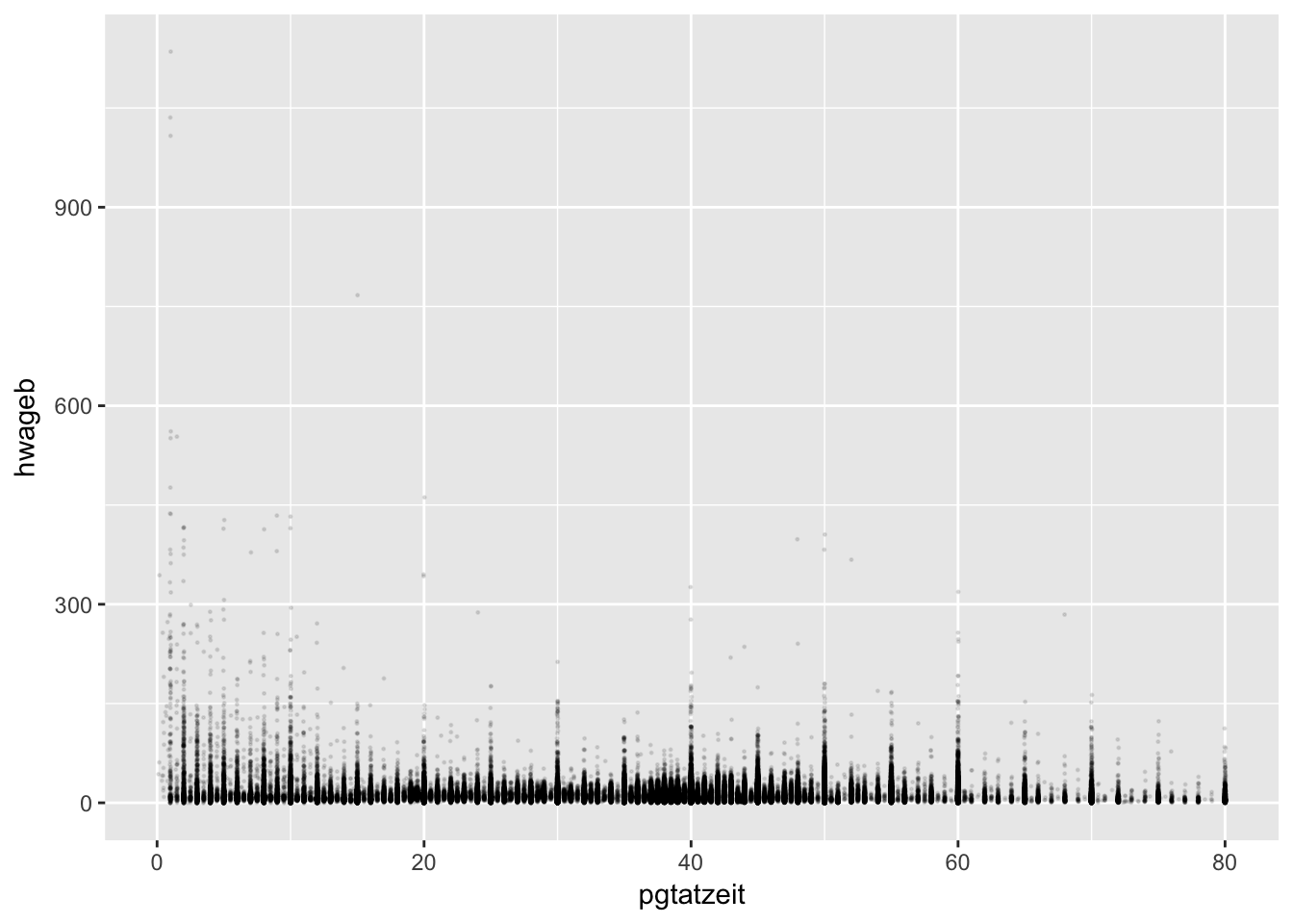
  # nochmal scatter
  ggplot(asample, aes(x=pgbilzeit, y=hwageb)) +
        geom_point(position = "jitter", size = 0.21, alpha = 0.1,
                   na.rm = T)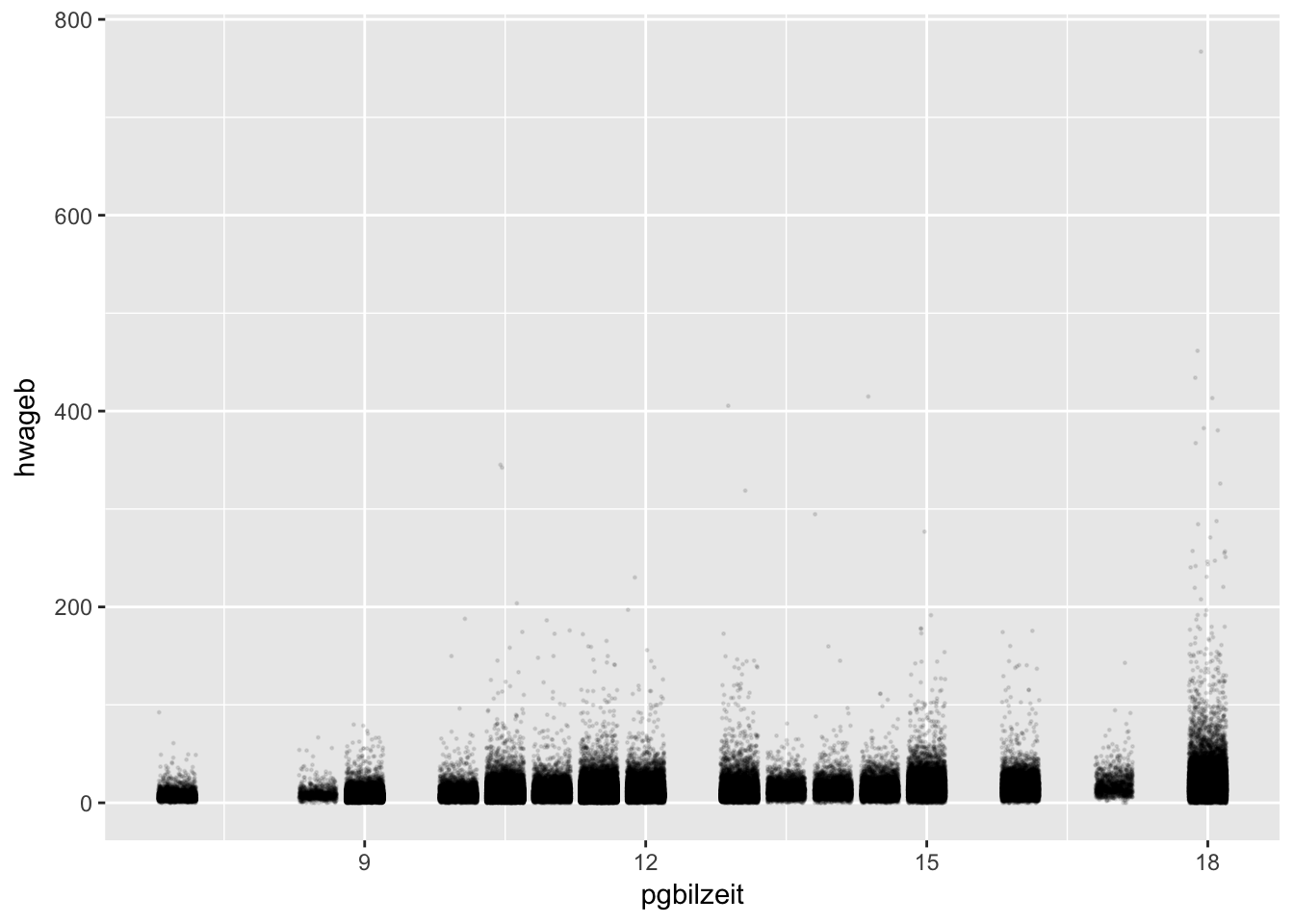
visualize Income
Here you can see three different ways to plot histograms in R: ###### Histogram
summary(asample$hwageb)## Min. 1st Qu. Median Mean 3rd Qu. Max. NA's
## 0 6 10 12 14 767 19# qplot
qplot(hwageb, geom="histogram",
binwidth = 25,
main = "Histogram for Hourly Wage",
xlab = "Hourly Wage in Prices from 2015",
fill=I("grey"),
col=I("black"),
alpha= I(.2),
xlim=c(0,500),
ylim= c(0,125000),
data = asample)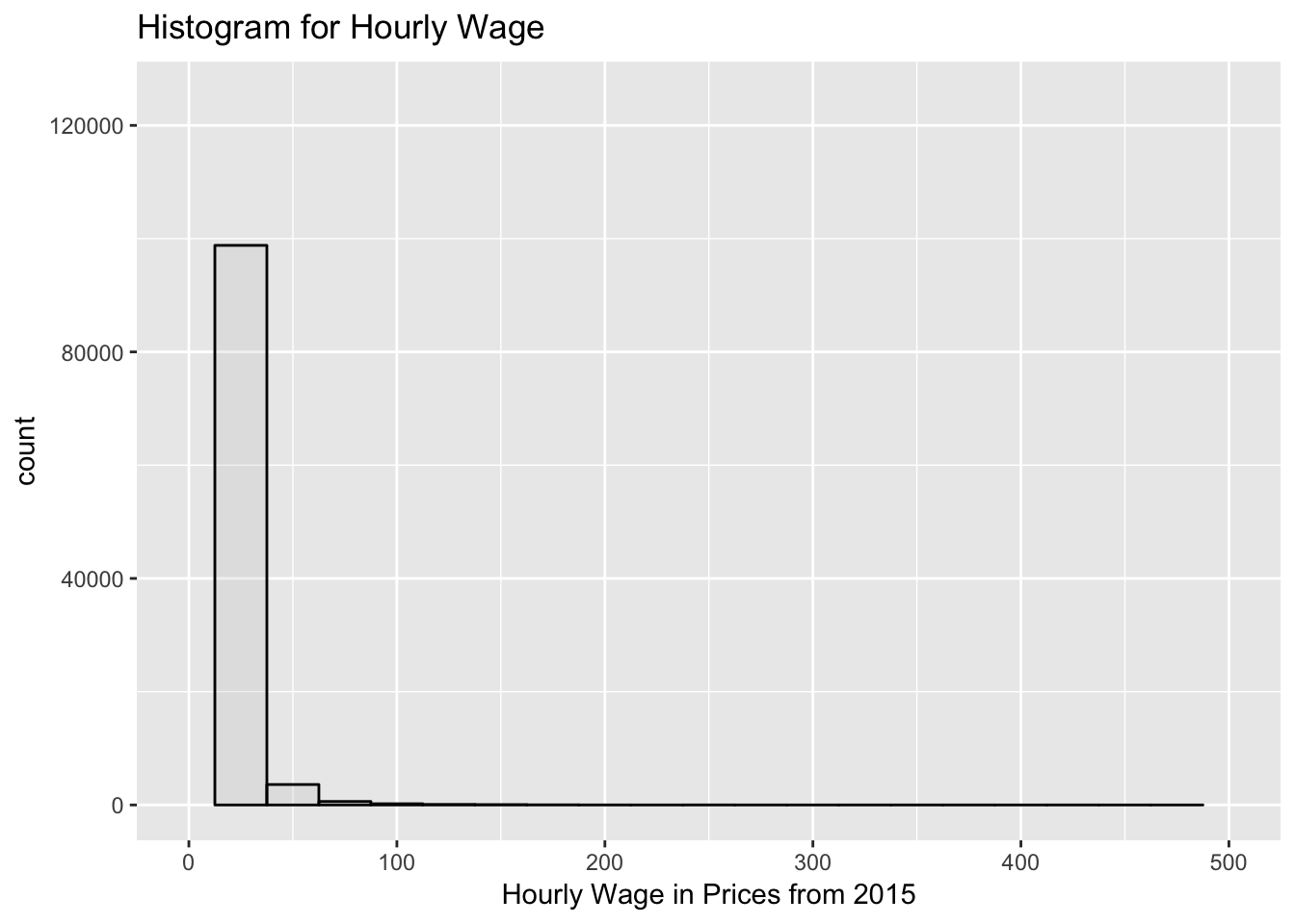
 # ggplot alternative
 # without ..density it would be counts
  g_hist_wage <- asample %>%
        ggplot(aes(x = hwageb, y = ..density..)) +
        geom_histogram(breaks = seq(0,767.4, by = 25)) +
        labs(title="Histogram for Hourly Wage in 2015 Prices",
             x="Hourly Wage")

  g_hist_wage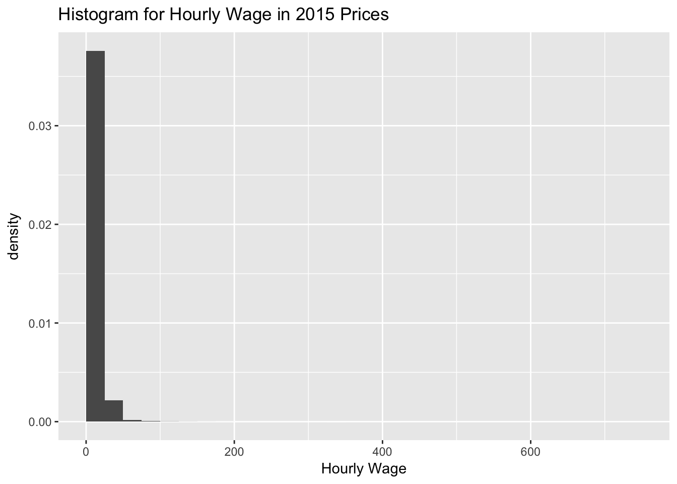
  # hist command
  hist(asample$hwageb, probability = T)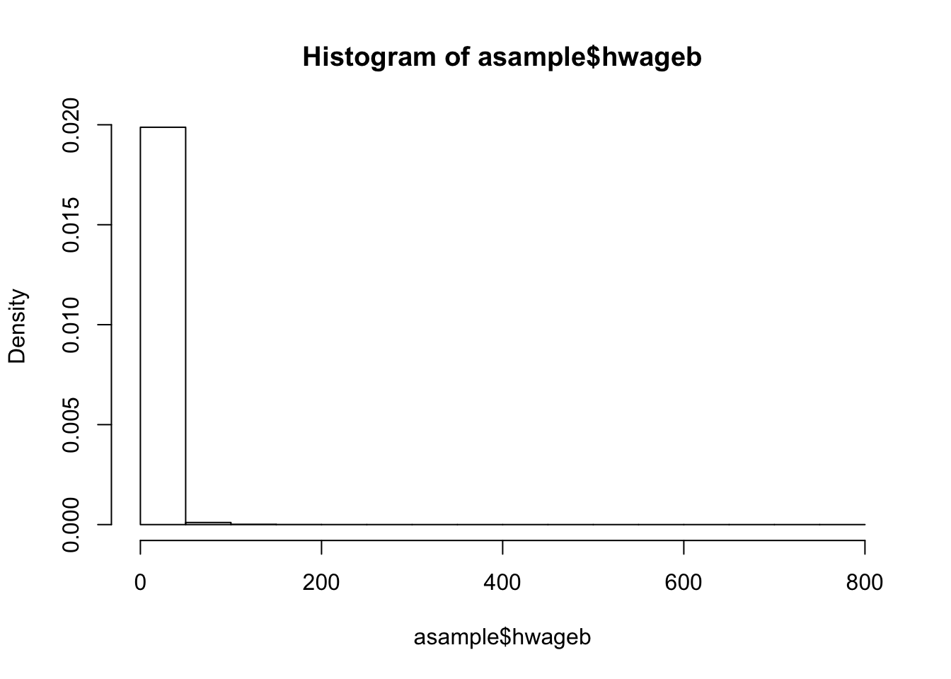
for 2015
summary of hourly wage and yrs of schooling, work exp, etc.
  asample %>%
      filter(syear == 2015) %>%
      select(hwageb, pgbilzeit, erf, frau, ost) %>%
      drop_na() %>%  # optional if complete.obs is specified
      cor(use = "complete.obs")
## hwageb pgbilzeit erf frau ost
## hwageb 1.00 0.366 0.210 -0.182 -0.113
## pgbilzeit 0.37 1.000 -0.104 0.037 0.042
## erf 0.21 -0.104 1.000 -0.275 0.075
## frau -0.18 0.037 -0.275 1.000 0.016
## ost -0.11 0.042 0.075 0.016 1.000 asample %>%
filter(syear == 2015) %>%
ggplot(aes(pgbilzeit, hwageb)) +
geom_point(na.rm=T, position = "jitter")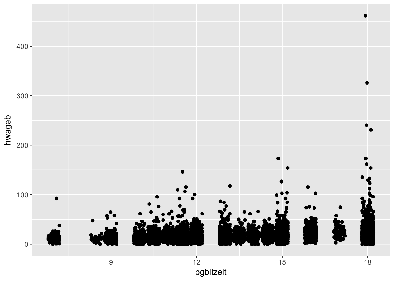
Answers
2.1 Basic Model
Estimate a Linear Regression with SOEP Data using hourly wage hwageb as dependent variable for the year 2015. Include years of schooling pgbilzeit and work experience erf as predictor variables and gender frau and region ost as additional controls.
Note: STATA command if e(sample): In STATA, there is a practical command if e(sample) that lets you restrict new calculations to the observations that were used in a model calculated before. In this exercise this can be used to calculate centralized coefficients for education and compare two models with each other, making sure that they are based on the same observations. In this exercise, the basic model is calculated first (2.1) and then another model is run with the same sample, but with centralized years of education and work experience (2.1c) in order to be able to interpret the intercept in a theoretically coherent way.
Note2: STATA - R Difference concerning weights in regression models. STATA and R handle weights with the value of 0 differently. While STATA drops these observations by default, R does not. In theory, weights of 0 should not exist, because sampling weights are supposed to be the inverse of the probability of being sampled. In survey data, sampling weights of 0 can be included because the weights are adjusted in various ways. If you want to include cases with 0 weights in STATA regressions you need to use the svy option as described here. If, on the other hand you want to exclude them from the R model, you can use a filter before modeling (e.g. filter(phrf > 0)). For the basic model in this exercise both ways are shown here (First without 0-weight observations, then with).
Stata
basic model
without weights0 cases:
  Linear regression                         Number of obs     =     14,218
                                            F(4, 14213)       =     259.84
                                            Prob > F          =     0.0000
                                            R-squared         =     0.2253
                                            Root MSE          =     10.072

  ------------------------------------------------------------------------------
               |               Robust
        hwageb |      Coef.   Std. Err.      t    P>|t|     [95% Conf. Interval]
  -------------+----------------------------------------------------------------
     pgbilzeit |   1.638184   .0619018    26.46   0.000     1.516848     1.75952
           erf |   .2431915   .0109426    22.22   0.000     .2217425    .2646405
          frau |  -2.754198   .2425546   -11.35   0.000    -3.229636   -2.278759
           ost |  -4.278906   .2718054   -15.74   0.000     -4.81168   -3.746132
         _cons |  -6.573576   .7699179    -8.54   0.000    -8.082716   -5.064436
  ------------------------------------------------------------------------------
Note: r markdown text with STATA output: Here is an example where I copied the output of the STATA regression into the R markdown in order to make it easy to compare it to the R output in the next tab. Because the STATA implementation in R markdown is not perfect yet, you cannot print single things in specific places but only run the code and see all of the output afterwards –> see tab “full code”. (This is partly due to the fact that R runs STATA from shell and certain features are not available there).
basic model II
with weights0 cases:
  Survey: Linear regression

  Number of strata   =         1                 Number of obs     =      14,300
  Number of PSUs     =    14,300                 Population size   =  33,885,938
                                                 Design df         =      14,299
                                                 F(   4,  14296)   =      259.86
                                                 Prob > F          =      0.0000
                                                 R-squared         =      0.2253

  ------------------------------------------------------------------------------
               |             Linearized
        hwageb |      Coef.   Std. Err.      t    P>|t|     [95% Conf. Interval]
  -------------+----------------------------------------------------------------
     pgbilzeit |   1.638184   .0618931    26.47   0.000     1.516866    1.759503
           erf |   .2431915   .0109411    22.23   0.000     .2217455    .2646375
          frau |  -2.754198   .2425205   -11.36   0.000    -3.229569   -2.278826
           ost |  -4.278906   .2717671   -15.74   0.000    -4.811605   -3.746207
         _cons |  -6.573576   .7698095    -8.54   0.000    -8.082503    -5.06465
  ------------------------------------------------------------------------------
Note: r markdown text with STATA output: Here is an example where I copied the output of the STATA regression into the R markdown in order to make it easy to compare it to the R output in the next tab. Because the STATA implementation in R markdown is not perfect yet, you cannot print single things in specific places but only run the code and see all of the output afterwards –> see tab “full code”. (This is partly due to the fact that R runs STATA from shell and certain features are not available there).
centered model
without weights0 cases:
  Linear regression                         Number of obs     =     14,218
                                            F(4, 14213)       =     259.84
                                            Prob > F          =     0.0000
                                            R-squared         =     0.2253
                                            Root MSE          =     10.072

  ------------------------------------------------------------------------------
               |               Robust
        hwageb |      Coef.   Std. Err.      t    P>|t|     [95% Conf. Interval]
  -------------+----------------------------------------------------------------
    cpgbilzeit |   1.638184   .0619018    26.46   0.000     1.516848     1.75952
          cerf |   .2431915   .0109426    22.22   0.000     .2217425    .2646405
          frau |  -2.754198   .2425546   -11.35   0.000    -3.229636   -2.278759
           ost |  -4.278906   .2718054   -15.74   0.000     -4.81168   -3.746132
         _cons |   18.51181   .2143393    86.37   0.000     18.09168    18.93194
  ------------------------------------------------------------------------------
Note: r markdown text with STATA output: Here is an example where I copied the output of the STATA regression into the R markdown in order to make it easy to compare it to the R output in the next tab. Because the STATA implementation in R markdown is not perfect yet, you cannot print single things in specific places but only run the code and see all of the output afterwards –> see tab “full code”. (This is partly due to the fact that R runs STATA from shell and certain features are not available there).
centered model II
with weights0 cases:
  Survey: Linear regression

  Number of strata   =         1                 Number of obs     =      14,300
  Number of PSUs     =    14,300                 Population size   =  33,885,938
                                                 Design df         =      14,299
                                                 F(   4,  14296)   =      259.86
                                                 Prob > F          =      0.0000
                                                 R-squared         =      0.2253

  ------------------------------------------------------------------------------
               |             Linearized
        hwageb |      Coef.   Std. Err.      t    P>|t|     [95% Conf. Interval]
  -------------+----------------------------------------------------------------
    cpgbilzeit |   1.638184   .0618931    26.47   0.000     1.516866    1.759503
          cerf |   .2431915   .0109411    22.23   0.000     .2217455    .2646374
          frau |  -2.754198   .2425205   -11.36   0.000    -3.229569   -2.278826
           ost |  -4.278906   .2717671   -15.74   0.000    -4.811605   -3.746207
         _cons |   18.51659   .2143495    86.39   0.000     18.09644    18.93674
  ------------------------------------------------------------------------------
Note: r markdown text with STATA output: Here is an example where I copied the output of the STATA regression into the R markdown in order to make it easy to compare it to the R output in the next tab. Because the STATA implementation in R markdown is not perfect yet, you cannot print single things in specific places but only run the code and see all of the output afterwards –> see tab “full code”. (This is partly due to the fact that R runs STATA from shell and certain features are not available there).
Full Code
use "_data/ex_mydf.dta", clear

* 2.1 basic model, no 0-weights
********************************************************************************
reg hwageb pgbilzeit erf frau ost if asample==1 & syear==2015 [pw=phrf]

* sum bildungszeit only for sample of last estimation
cap drop cpgbilzeit
sum pgbilzeit if e(sample)
gen cpgbilzeit = pgbilzeit - r(mean)

cap drop cerf
sum erf if e(sample)
gen cerf = erf -r(mean)

sum pgbilzeit cpgbilzeit if e(sample)
sum erf cerf if e(sample)

* 2.1c model with centered predictors, no 0-weights
reg hwageb cpgbilzeit cerf frau ost if asample==1 & syear==2015 [pw=phrf]


* 2.1 basic model, with 0-weights
********************************************************************************
svyset [pw=phrf]

svy: reg hwageb pgbilzeit erf frau ost if asample==1 & syear==2015

* sum bildungszeit only for sample of last estimation
cap drop cpgbilzeit
sum pgbilzeit if e(sample)
gen cpgbilzeit = pgbilzeit - r(mean)

cap drop cerf
sum erf if e(sample)
gen cerf = erf -r(mean)

sum pgbilzeit cpgbilzeit if e(sample)
sum erf cerf if e(sample)

* 2.1c model with centered predictors, with 0-weights
svy: reg hwageb cpgbilzeit cerf frau ost if asample==1 & syear==2015
. use "_data/ex_mydf.dta", clear
(PGEN: Feb 12, 2017 13:00:53-1 DBV32L)

.
. * 2.1 basic model, no 0-weights
. *****************************************************************************
> ***
. reg hwageb pgbilzeit erf frau ost if asample==1 & syear==2015 [pw=phrf]
(sum of wgt is   3.3886e+07)

Linear regression                               Number of obs     =     14,218
                                                F(4, 14213)       =     259.84
                                                Prob > F          =     0.0000
                                                R-squared         =     0.2253
                                                Root MSE          =     10.072

------------------------------------------------------------------------------
             |               Robust
      hwageb |      Coef.   Std. Err.      t    P>|t|     [95% Conf. Interval]
-------------+----------------------------------------------------------------
   pgbilzeit |   1.638184   .0619018    26.46   0.000     1.516848     1.75952
         erf |   .2431915   .0109426    22.22   0.000     .2217425    .2646405
        frau |  -2.754198   .2425546   -11.35   0.000    -3.229636   -2.278759
         ost |  -4.278906   .2718054   -15.74   0.000     -4.81168   -3.746132
       _cons |  -6.573576   .7699179    -8.54   0.000    -8.082716   -5.064436
------------------------------------------------------------------------------

.
. * sum bildungszeit only for sample of last estimation
. cap drop cpgbilzeit

. sum pgbilzeit if e(sample)

    Variable |        Obs        Mean    Std. Dev.       Min        Max
-------------+---------------------------------------------------------
   pgbilzeit |     14,218    12.85849     2.77797          7         18

. gen cpgbilzeit = pgbilzeit - r(mean)
(27,340 missing values generated)

.
. cap drop cerf

. sum erf if e(sample)

    Variable |        Obs        Mean    Std. Dev.       Min        Max
-------------+---------------------------------------------------------
         erf |     14,218    16.53353    10.91589          0      64.48

. gen cerf = erf -r(mean)
(13,804 missing values generated)

.
. sum pgbilzeit cpgbilzeit if e(sample)

    Variable |        Obs        Mean    Std. Dev.       Min        Max
-------------+---------------------------------------------------------
   pgbilzeit |     14,218    12.85849     2.77797          7         18
  cpgbilzeit |     14,218    1.03e-08     2.77797  -5.858489   5.141511

. sum erf cerf if e(sample)

    Variable |        Obs        Mean    Std. Dev.       Min        Max
-------------+---------------------------------------------------------
         erf |     14,218    16.53353    10.91589          0      64.48
        cerf |     14,218    1.35e-07    10.91589  -16.53353   47.94647

.
. * 2.1c model with centered predictors, no 0-weights
. reg hwageb cpgbilzeit cerf frau ost if asample==1 & syear==2015 [pw=phrf]
(sum of wgt is   3.3886e+07)

Linear regression                               Number of obs     =     14,218
                                                F(4, 14213)       =     259.84
                                                Prob > F          =     0.0000
                                                R-squared         =     0.2253
                                                Root MSE          =     10.072

------------------------------------------------------------------------------
             |               Robust
      hwageb |      Coef.   Std. Err.      t    P>|t|     [95% Conf. Interval]
-------------+----------------------------------------------------------------
  cpgbilzeit |   1.638184   .0619018    26.46   0.000     1.516848     1.75952
        cerf |   .2431915   .0109426    22.22   0.000     .2217425    .2646405
        frau |  -2.754198   .2425546   -11.35   0.000    -3.229636   -2.278759
         ost |  -4.278906   .2718054   -15.74   0.000     -4.81168   -3.746132
       _cons |   18.51181   .2143393    86.37   0.000     18.09168    18.93194
------------------------------------------------------------------------------

.
.
. * 2.1 basic model, with 0-weights
. *****************************************************************************
> ***
. svyset [pw=phrf]

      pweight: phrf
          VCE: linearized
  Single unit: missing
     Strata 1: <one>
         SU 1: <observations>
        FPC 1: <zero>

.
. svy: reg hwageb pgbilzeit erf frau ost if asample==1 & syear==2015
(running regress on estimation sample)

Survey: Linear regression

Number of strata   =         1                 Number of obs     =      14,300
Number of PSUs     =    14,300                 Population size   =  33,885,938
                                               Design df         =      14,299
                                               F(   4,  14296)   =      259.86
                                               Prob > F          =      0.0000
                                               R-squared         =      0.2253

------------------------------------------------------------------------------
             |             Linearized
      hwageb |      Coef.   Std. Err.      t    P>|t|     [95% Conf. Interval]
-------------+----------------------------------------------------------------
   pgbilzeit |   1.638184   .0618931    26.47   0.000     1.516866    1.759503
         erf |   .2431915   .0109411    22.23   0.000     .2217455    .2646375
        frau |  -2.754198   .2425205   -11.36   0.000    -3.229569   -2.278826
         ost |  -4.278906   .2717671   -15.74   0.000    -4.811605   -3.746207
       _cons |  -6.573576   .7698095    -8.54   0.000    -8.082503    -5.06465
------------------------------------------------------------------------------

.
. * sum bildungszeit only for sample of last estimation
. cap drop cpgbilzeit

. sum pgbilzeit if e(sample)

    Variable |        Obs        Mean    Std. Dev.       Min        Max
-------------+---------------------------------------------------------
   pgbilzeit |     14,297    12.85934    2.777205          7         18

. gen cpgbilzeit = pgbilzeit - r(mean)
(27,340 missing values generated)

.
. cap drop cerf

. sum erf if e(sample)

    Variable |        Obs        Mean    Std. Dev.       Min        Max
-------------+---------------------------------------------------------
         erf |     14,299    16.54744    10.91855          0      64.48

. gen cerf = erf -r(mean)
(13,804 missing values generated)

.
. sum pgbilzeit cpgbilzeit if e(sample)

    Variable |        Obs        Mean    Std. Dev.       Min        Max
-------------+---------------------------------------------------------
   pgbilzeit |     14,297    12.85934    2.777205          7         18
  cpgbilzeit |     14,297   -2.28e-08    2.777205  -5.859341   5.140659

. sum erf cerf if e(sample)

    Variable |        Obs        Mean    Std. Dev.       Min        Max
-------------+---------------------------------------------------------
         erf |     14,299    16.54744    10.91855          0      64.48
        cerf |     14,299   -8.50e-08    10.91855  -16.54744   47.93256

.
. * 2.1c model with centered predictors, with 0-weights
. svy: reg hwageb cpgbilzeit cerf frau ost if asample==1 & syear==2015
(running regress on estimation sample)

Survey: Linear regression

Number of strata   =         1                 Number of obs     =      14,300
Number of PSUs     =    14,300                 Population size   =  33,885,938
                                               Design df         =      14,299
                                               F(   4,  14296)   =      259.86
                                               Prob > F          =      0.0000
                                               R-squared         =      0.2253

------------------------------------------------------------------------------
             |             Linearized
      hwageb |      Coef.   Std. Err.      t    P>|t|     [95% Conf. Interval]
-------------+----------------------------------------------------------------
  cpgbilzeit |   1.638184   .0618931    26.47   0.000     1.516866    1.759503
        cerf |   .2431915   .0109411    22.23   0.000     .2217455    .2646374
        frau |  -2.754198   .2425205   -11.36   0.000    -3.229569   -2.278826
         ost |  -4.278906   .2717671   -15.74   0.000    -4.811605   -3.746207
       _cons |   18.51659   .2143495    86.39   0.000     18.09644    18.93674
------------------------------------------------------------------------------
R
Models
basic model
without weights0 cases
# fit regression model
  # automatically drops rows with missing values
  fit2.1_no0w <- asample15 %>%
      # filter sample weights = 0
      filter(phrf > 0) %>%
      lm(hwageb ~ pgbilzeit + erf + frau + ost,
         data= ., weights = phrf)

  tidy(fit2.1_no0w, conf.int = T)
glance(fit2.1_no0w) # summary(fit2.1_no0w)
# with robust standard errors
tidy(coeftest(fit2.1_no0w, vcov = vcovHC(fit2.1_no0w, "HC1"))) # robust; HC1 (Stata default)basic model II
with weights0 cases
# fit regression model
  # automatically drops rows with missing values
  fit2.1 <- asample15 %>%
      lm(hwageb ~ pgbilzeit + erf + frau + ost,
         data= ., weights = phrf)

  tidy(fit2.1, conf.int = T)
glance(fit2.1) # summary(fit2.1)
coeftest(fit2.1, vcov = vcovHC(fit2.1, "HC1")) # robust; HC1 (Stata default)##
## t test of coefficients:
##
## Estimate Std. Error t value Pr(>|t|)
## (Intercept) -6.5736 0.7657 -8.59 <2e-16 ***
## pgbilzeit 1.6382 0.0616 26.61 <2e-16 ***
## erf 0.2432 0.0109 22.35 <2e-16 ***
## frau -2.7542 0.2412 -11.42 <2e-16 ***
## ost -4.2789 0.2703 -15.83 <2e-16 ***
## ---
## Signif. codes: 0 '***' 0.001 '**' 0.01 '*' 0.05 '.' 0.1 ' ' 1centered model
without weights0 cases
with centralized years of schooling and work experience. This can be helpful to interpret the intercept, because 0 years education are not a realistic interpretation
Note: STATA command if e(sample) implementation in R. In order to achieve the same effect of the if e(sample) addition in STATA, one can store the rownames of the observations in the fitted model and use these to filter the dataset that the next model is based on (or for whichever computation this restriction is needed).
esample <- rownames(as.matrix(resid((fit2.1_no0w))))

# regress again with centered predictors
fit2.1c_no0w <-  asample15 %>%
  # filter only obs used in last model
  filter(row_number() %in% esample) %>%
  # centralized values for education by year
  mutate(cpgbilzeit = pgbilzeit - mean(pgbilzeit, na.rm = T),
         cerf = erf - mean(erf, na.rm = T)) %>%
  # linear model
  lm(hwageb ~ cpgbilzeit + cerf + frau + ost,
     data= ., weights = phrf)

  tidy(fit2.1c_no0w)
coeftest(fit2.1c_no0w, vcov = vcovHC(fit2.1c_no0w, "HC1")) # robust; HC1 (Stata default)##
## t test of coefficients:
##
## Estimate Std. Error t value Pr(>|t|)
## (Intercept) 18.5457 0.2169 85.5 <2e-16 ***
## cpgbilzeit 1.6350 0.0625 26.2 <2e-16 ***
## cerf 0.2420 0.0110 21.9 <2e-16 ***
## frau -2.8154 0.2452 -11.5 <2e-16 ***
## ost -4.3037 0.2744 -15.7 <2e-16 ***
## ---
## Signif. codes: 0 '***' 0.001 '**' 0.01 '*' 0.05 '.' 0.1 ' ' 1 # Sample identifier, a set of row names which can be used to subset the corresponding dataframeNumber of Observations in the sample
length(esample)## [1] 14218centered model II
with weights0 cases
# Sample identifier, a set of row names which can be used to subset the corresponding dataframe
esample <- rownames(as.matrix(resid((fit2.1))))

# regress again with centered predictors
fit2.1c <-  asample15 %>%
  # filter only obs used in last model
  filter(row_number() %in% esample) %>%
  # generate centralized values for education by year
  mutate(cpgbilzeit = pgbilzeit - mean(pgbilzeit, na.rm = T),
         cerf = erf - mean(erf, na.rm = T)) %>%
  # linear model
  lm(hwageb ~ cpgbilzeit + cerf + frau + ost,
     data= ., weights = phrf)

  tidy(fit2.1c)
coeftest(fit2.1c, vcov = vcovHC(fit2.1c, "HC1")) # robust; HC1 (Stata default)##
## t test of coefficients:
##
## Estimate Std. Error t value Pr(>|t|)
## (Intercept) 18.5170 0.2132 86.8 <2e-16 ***
## cpgbilzeit 1.6382 0.0616 26.6 <2e-16 ***
## cerf 0.2432 0.0109 22.4 <2e-16 ***
## frau -2.7542 0.2412 -11.4 <2e-16 ***
## ost -4.2789 0.2703 -15.8 <2e-16 ***
## ---
## Signif. codes: 0 '***' 0.001 '**' 0.01 '*' 0.05 '.' 0.1 ' ' 1 # summary statistics of education and job experience with sample of last regression
asample15 %>%
filter(row_number() %in% esample) %>% # this needs to be in a separate filter, otherwise wont work
select(pgbilzeit, erf) %>%
stat.desc(basic = T)Number of Observations in the sample
length(esample)## [1] 14297Plots
# plot it
  asample %>%
      filter(syear == 2015) %>%
      ggplot(aes(pgbilzeit, hwageb)) +
      geom_point() +
      geom_smooth(method="lm", color="red", se=F) +
      geom_line(aes(y = mean(asample$hwageb)), color="blue")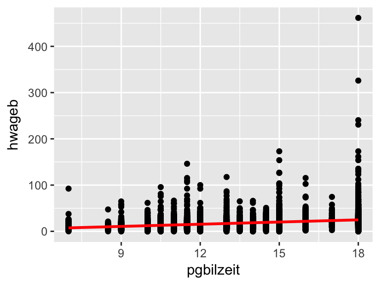
This code produces a set of four plots: residuals versus fitted values, a Q-Q plot of standardized residuals, a scale-location plot (square roots of standardized residuals versus fitted values) and a plot of residuals versus leverage that adds bands corresponding to Cook’s distances of 0.5 and 1. The par option is specified, in order to display all four of them at once and not in separate steps. This option is revoked afterwards. You can type ?par into R to learn more.
par(mfrow=c(2,2))
plot(fit2.1)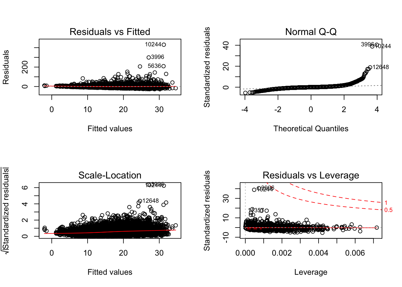
par(mfrow=c(1,1))More Info
More Information about single parts of the model(s).
These are quick ways to extract the confidence intervals, intercept and slopes of a model:
# extract Confidence Intervals
      confint(fit2.1)
## 2.5 % 97.5 %
## (Intercept) -7.48 -5.66
## pgbilzeit 1.58 1.70
## erf 0.23 0.26
## frau -3.09 -2.41
## ost -4.71 -3.84# extract intercept
fit2.1$coef[1]## (Intercept)
## -6.6# extract slope
fit2.1$coef[2:5]## pgbilzeit erf frau ost
## 1.64 0.24 -2.75 -4.28# extract the names of the content in your model
names(fit2.1)## [1] "coefficients" "residuals" "fitted.values" "effects"
## [5] "weights" "rank" "assign" "qr"
## [9] "df.residual" "na.action" "xlevels" "call"
## [13] "terms" "model"2.2 coefficients and R²
Interpret the coefficients and the value of R²
Model 2.1 Coefficients
- Intercept
The intercept is negative, which does not make theoretical sense because wages cannot be negative. Mathematically it reflects the predicted value if all explanatory variables are equal to 0. Since there is “Schulpflicht” in Germany, it is not the case that there are people with no education at all in the dataset. Since there are no observations with education < 7, the model cannot predict those cases successfully. In order to be able to interpret the intercept after all, one can center the variables.
- Years of Education (
pgbilzeit)- For each unit (year) increase of education, hourly wage is expected to increase by 1.64 units (Euro).
- Work Experience (
erf)- For each increase of working experience by one year, the expects income increases by 0,24 Euro/hour.
- Gender (
frau)- Women are expected to earn 2.75 Euro less per hour compared to men.
- Region (
ost)- People who grew up in former eastern germany are estimated to earn 4.26 Euro less, compared to people who grew up in former western Germany.
- R-squared
- The model can explain 22.59% of the overall variance of hourly wages in Germany.
Model 2.1c Coefficients
- Intercept
With the variables education and work experience centered, one can interpret the intercept as: For male Germans (
frau== 0) who were born in former West Germany (ost== 0) and with average years of education (cpgbilzeit) and average years of work experience (cerf), the expected hourly wage is 18,51 Euro/h.One can now also predict the wages for other groups by adding the values of the coefficients and the intercept. E.g. The model predicts hourly wages of
18.51 - 2.75 = 15.76Euro/h for females compared to 18.51 Euro/h for males, holding education and work experience equal.
2.3 work experience and wage
Is the relationship between work experience and wage linear?
Labor market research found that the relationship of work and wage is not linear. In the cprplots one can see the that model that assumes linearity systematically overestimates people with long work experience. The solution to this would be to use the squared term of work experience in the model.
Stata
Models
use "_data/ex_mydf.dta", clear

    reg hwageb i.frau pgbilzeit erf ost if asample==1 & syear==2015 [pw=phrf]

    cprplot erf, msize(vsmall) jitter(2) mspline msopts(bands(11) lcolor(red)) name(cpr_2_3, replace)

    *graph use cpr_2_3
    *graph export "out/cpr_2_3.png", replace

      reg hwageb i.frau##c.pgbilzeit c.erf##c.erf ost if asample==1 & syear==2015 [pw=phrf]
    cprplot erf, msize(vsmall) jitter(2) mspline msopts(bands(11) lcolor(red)) name(cpr_2_32, replace)

    *graph use cpr_2_32
    *graph export "out/cpr_2_32.png", replace
.
. use "_data/ex_mydf.dta", clear
(PGEN: Feb 12, 2017 13:00:53-1 DBV32L)

.
.         reg hwageb i.frau pgbilzeit erf ost if asample==1 & syear==2015 [pw=p
> hrf]
(sum of wgt is   3.3886e+07)

Linear regression                               Number of obs     =     14,218
                                                F(4, 14213)       =     259.84
                                                Prob > F          =     0.0000
                                                R-squared         =     0.2253
                                                Root MSE          =     10.072

------------------------------------------------------------------------------
             |               Robust
      hwageb |      Coef.   Std. Err.      t    P>|t|     [95% Conf. Interval]
-------------+----------------------------------------------------------------
        frau |
   weiblich  |  -2.754198   .2425546   -11.35   0.000    -3.229636   -2.278759
   pgbilzeit |   1.638184   .0619018    26.46   0.000     1.516848     1.75952
         erf |   .2431915   .0109426    22.22   0.000     .2217425    .2646405
         ost |  -4.278906   .2718054   -15.74   0.000     -4.81168   -3.746132
       _cons |  -6.573576   .7699179    -8.54   0.000    -8.082716   -5.064436
------------------------------------------------------------------------------

.
.         cprplot erf, msize(vsmall) jitter(2) mspline msopts(bands(11) lcolor(
> red)) name(cpr_2_3, replace)

.
.         *graph use cpr_2_3
.         *graph export "out/cpr_2_3.png", replace
.
.       reg hwageb i.frau##c.pgbilzeit c.erf##c.erf ost if asample==1 & syear==
> 2015 [pw=phrf]
(sum of wgt is   3.3886e+07)

Linear regression                               Number of obs     =     14,218
                                                F(6, 14211)       =     241.95
                                                Prob > F          =     0.0000
                                                R-squared         =     0.2375
                                                Root MSE          =     9.9937

------------------------------------------------------------------------------
             |               Robust
      hwageb |      Coef.   Std. Err.      t    P>|t|     [95% Conf. Interval]
-------------+----------------------------------------------------------------
        frau |
   weiblich  |   2.018305   1.339491     1.51   0.132    -.6072725    4.643882
   pgbilzeit |   1.790837   .0980965    18.26   0.000     1.598556    1.983119
             |
        frau#|
 c.pgbilzeit |
   weiblich  |  -.3821273    .113354    -3.37   0.001     -.604316   -.1599387
             |
         erf |   .5718543   .0346963    16.48   0.000     .5038451    .6398636
             |
 c.erf#c.erf |  -.0084294   .0008973    -9.39   0.000    -.0101881   -.0066707
             |
         ost |   -4.15973   .2665798   -15.60   0.000    -4.682261   -3.637198
       _cons |  -10.53201    1.21738    -8.65   0.000    -12.91823   -8.145781
------------------------------------------------------------------------------

.         cprplot erf, msize(vsmall) jitter(2) mspline msopts(bands(11) lcolor(
> red)) name(cpr_2_32, replace)

.
.         *graph use cpr_2_32
.         *graph export "out/cpr_2_32.png", replace
.
Plots
Component + Residual Plot
knitr::include_graphics("out/cpr_2_3.png")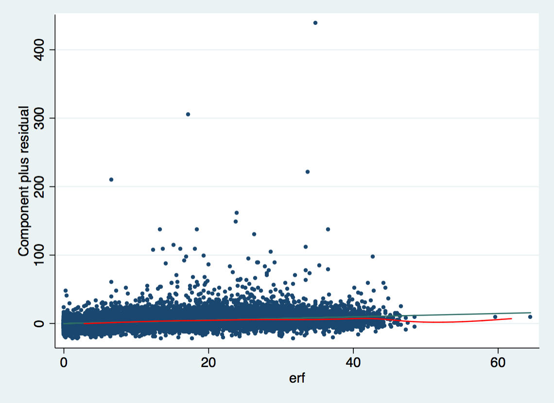
Component + Residual Plot with squared work experience
knitr::include_graphics("out/cpr_2_32.png")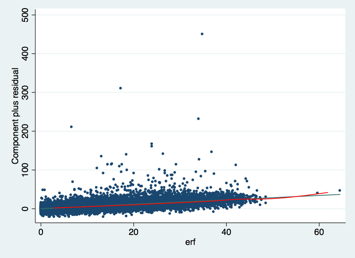
R
Models
Base Model
# base model
  fit2.3 <- asample%>%
      filter(syear == 2015) %>%
      lm(hwageb ~ frau + pgbilzeit + erf + ost,
                      data= ., weights = phrf)

  tidy(fit2.3)
Model with squared experience
  fit2.3_exp <- asample %>%
       filter(syear == 2015) %>%
       mutate(frau.d = factor(frau)) %>%
       lm(hwageb ~ frau + pgbilzeit + erf + I(erf^2) + ost,
          data= ., weights = phrf)

  tidy(fit2.3_exp)
Plots
Component + Residual Plot Note: These plots are not available if there is an interaction term in the model formula. It does work, if the interaction term is stored in an extra variable.
crPlots(fit2.3, terms = .~ erf, layout = c(1,1)) # from car package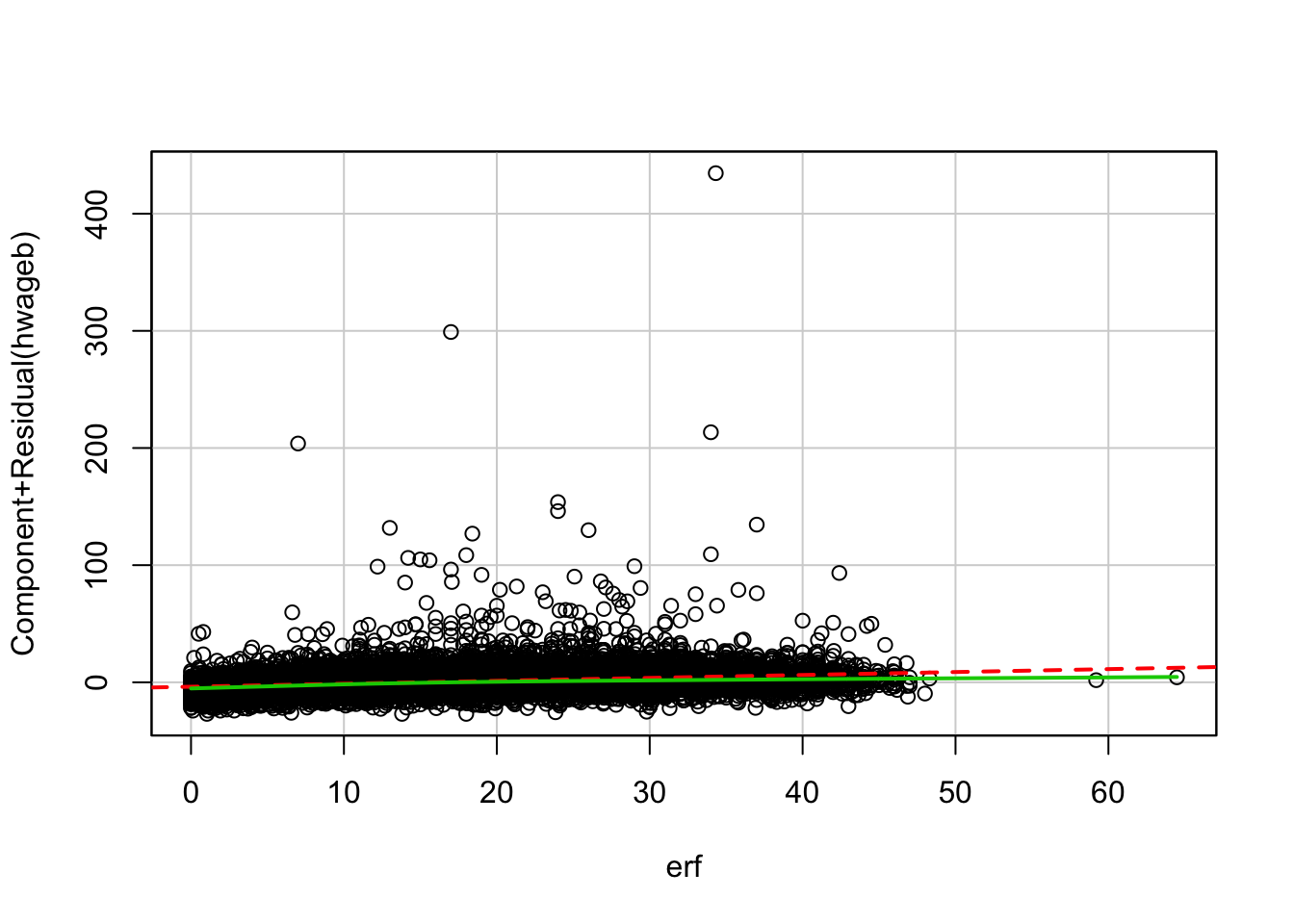
Component + Residual Plot with squared work experience
fit2.3_exp <- asample %>%
       filter(syear == 2015) %>%
       mutate(erfq = erf*erf) %>%
       lm(hwageb ~ frau + pgbilzeit + erf + erfq + ost,
          data= ., weights = phrf)

 crPlots(fit2.3_exp, terms = .~ erf, layout = c(1,1))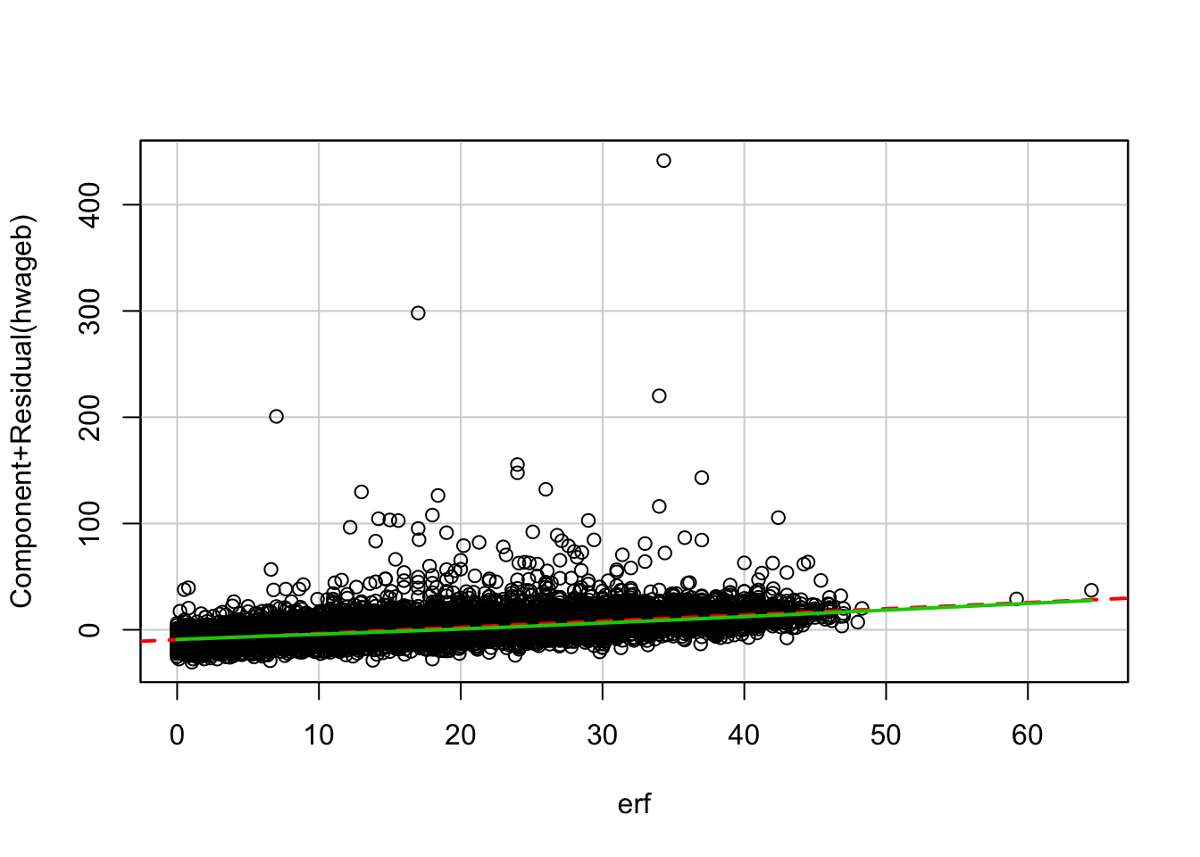
2.4 Log Model
Specifiy the same regression model but use the natural logarithm as dependent variable instead. How does the the interpretation of coefficients change?
Why use log of wage? The distribution of hourly wage is very right skewed while the log(wage) is closer to a normal distribution. Since the dependent variable is now the natural logarithm, it is not very intuitive to interpret.
How does the the interpretation of coefficients change?
- Now that we calculate a Log-Level-Effect the coefficient of x would stand for the change in ln(y), if x changes by one unit. In order to be better able to interpret the coefficients, we can interpret the exponential form of the model. Then the coefficient of x by one unit stands for \(e^b\). The coefficients can now be interpreted as percentage change.
Stata
use "_data/ex_mydf.dta", clear

* Mincer-Equation
    reg lnwage pgbilzeit erf frau ost if asample==1 & syear==2015 [pw=phrf]

      dis exp(.0868897)
      dis  .3956569^2
.
. use "_data/ex_mydf.dta", clear
(PGEN: Feb 12, 2017 13:00:53-1 DBV32L)

.
. * Mincer-Equation
.         reg lnwage pgbilzeit erf frau ost if asample==1 & syear==2015 [pw=phr
> f]
(sum of wgt is   3.3697e+07)

Linear regression                               Number of obs     =     14,150
                                                F(4, 14145)       =     460.46
                                                Prob > F          =     0.0000
                                                R-squared         =     0.2787
                                                Root MSE          =     .48652

------------------------------------------------------------------------------
             |               Robust
      lnwage |      Coef.   Std. Err.      t    P>|t|     [95% Conf. Interval]
-------------+----------------------------------------------------------------
   pgbilzeit |   .0871554   .0027229    32.01   0.000     .0818181    .0924928
         erf |   .0150668   .0006599    22.83   0.000     .0137733    .0163604
        frau |  -.1350645   .0140727    -9.60   0.000    -.1626489   -.1074801
         ost |   -.270033   .0178111   -15.16   0.000    -.3049452   -.2351209
       _cons |   1.390662   .0408833    34.02   0.000     1.310525    1.470798
------------------------------------------------------------------------------

.
.       dis exp(.0868897)
1.0907764

.       dis  .3956569^2
.15654438
R
Model
 fit2.4 <- asample15 %>%
        lm(lnwage ~ pgbilzeit + erf + frau + ost,
           data = ., weights = phrf)

tidy(fit2.4, conf.int = T) glance(fit2.4)Interpretation of coefficients Example coefficient for education: exp(.0871554) = 1.09 -> for every increase of education by one unit (year), wage grows by 9%
exp(.0871554) ## [1] 1.1If you want to know the change of 8 years more education: exp(.0871554)^8 = 2,01 -> 101% increase
exp(.0871554)^8 ## [1] 22.5 Gender Pay Gap
How large is the gender pay gap?
Stata
use "_data/ex_mydf.dta", clear

* raw gap
reg lnwage frau if asample==1 & syear==2015 [pw=phrf]
dis exp(-.1983373)

* gender wage gap 2015
reg lnwage pgbilzeit c.erf##c.erf i.frau i.ost if asample==1 & syear == 2015 [pw=phrf]

dis exp(-.1456176)
. use "_data/ex_mydf.dta", clear
(PGEN: Feb 12, 2017 13:00:53-1 DBV32L)

.
. * raw gap
. reg lnwage frau if asample==1 & syear==2015 [pw=phrf]
(sum of wgt is   3.5427e+07)

Linear regression                               Number of obs     =     14,691
                                                F(1, 14689)       =     169.09
                                                Prob > F          =     0.0000
                                                R-squared         =     0.0297
                                                Root MSE          =     .56728

------------------------------------------------------------------------------
             |               Robust
      lnwage |      Coef.   Std. Err.      t    P>|t|     [95% Conf. Interval]
-------------+----------------------------------------------------------------
        frau |   -.198841   .0152913   -13.00   0.000    -.2288138   -.1688682
       _cons |   2.754187   .0112659   244.47   0.000     2.732105     2.77627
------------------------------------------------------------------------------

. dis exp(-.1983373)
.82009319

.
. * gender wage gap 2015
. reg lnwage pgbilzeit c.erf##c.erf i.frau i.ost if asample==1 & syear == 2015
> [pw=phrf]
(sum of wgt is   3.3697e+07)

Linear regression                               Number of obs     =     14,150
                                                F(5, 14144)       =     391.34
                                                Prob > F          =     0.0000
                                                R-squared         =     0.2969
                                                Root MSE          =     .48037

------------------------------------------------------------------------------
             |               Robust
      lnwage |      Coef.   Std. Err.      t    P>|t|     [95% Conf. Interval]
-------------+----------------------------------------------------------------
   pgbilzeit |   .0856499   .0026784    31.98   0.000     .0803999    .0908999
         erf |   .0381035   .0022446    16.98   0.000     .0337039    .0425032
             |
 c.erf#c.erf |  -.0005924   .0000521   -11.36   0.000    -.0006946   -.0004902
             |
        frau |
   weiblich  |  -.1456176   .0137884   -10.56   0.000    -.1726446   -.1185906
             |
         ost |
        Ost  |  -.2642993   .0176628   -14.96   0.000    -.2989206   -.2296779
       _cons |   1.270545   .0429209    29.60   0.000     1.186414    1.354675
------------------------------------------------------------------------------

.
. dis exp(-.1456176)
.86448822
R
Models
raw gap
fit2.5_raw <- asample15 %>%
        lm(lnwage ~  frau , data = ., weights = phrf)

tidy(fit2.5_raw, conf.int=T)
Effect of gender on wage Compared to males, wages for females change by a factor of 0.8197, in other words are diminished by 18.03 %
exp(fit2.5_raw$coefficients["frau"])## frau
## 0.821 - exp(fit2.5_raw$coefficients["frau"])## frau
## 0.18Wage gap with further coefficients
fit2.5 <- asample15 %>%
        lm(lnwage ~ pgbilzeit + I(erf^2) + frau + ost,
           data = ., weights = phrf)

tidy(fit2.5)
Compared to males, wages for females change by a factor of 0.8197, in other words are diminished by 13.39 %
exp(fit2.5$coefficients["frau"])## frau
## 0.861 - exp(fit2.5$coefficients["frau"])## frau
## 0.14