Stata
use "_data/ess50.dta", clear

xtmixed stfdem polintr nwsptot gndr || cntry:
estat icc
. use "_data/ess50.dta", clear
.
. xtmixed stfdem polintr nwsptot gndr || cntry:
Performing EM optimization:
Performing gradient-based optimization:
Iteration 0: log likelihood = -24314.832
Iteration 1: log likelihood = -24314.832
Computing standard errors:
Mixed-effects ML regression Number of obs = 10,963
Group variable: cntry Number of groups = 22
Obs per group:
min = 46
avg = 498.3
max = 1,544
Wald chi2(3) = 110.94
Log likelihood = -24314.832 Prob > chi2 = 0.0000
------------------------------------------------------------------------------
stfdem | Coef. Std. Err. z P>|z| [95% Conf. Interval]
-------------+----------------------------------------------------------------
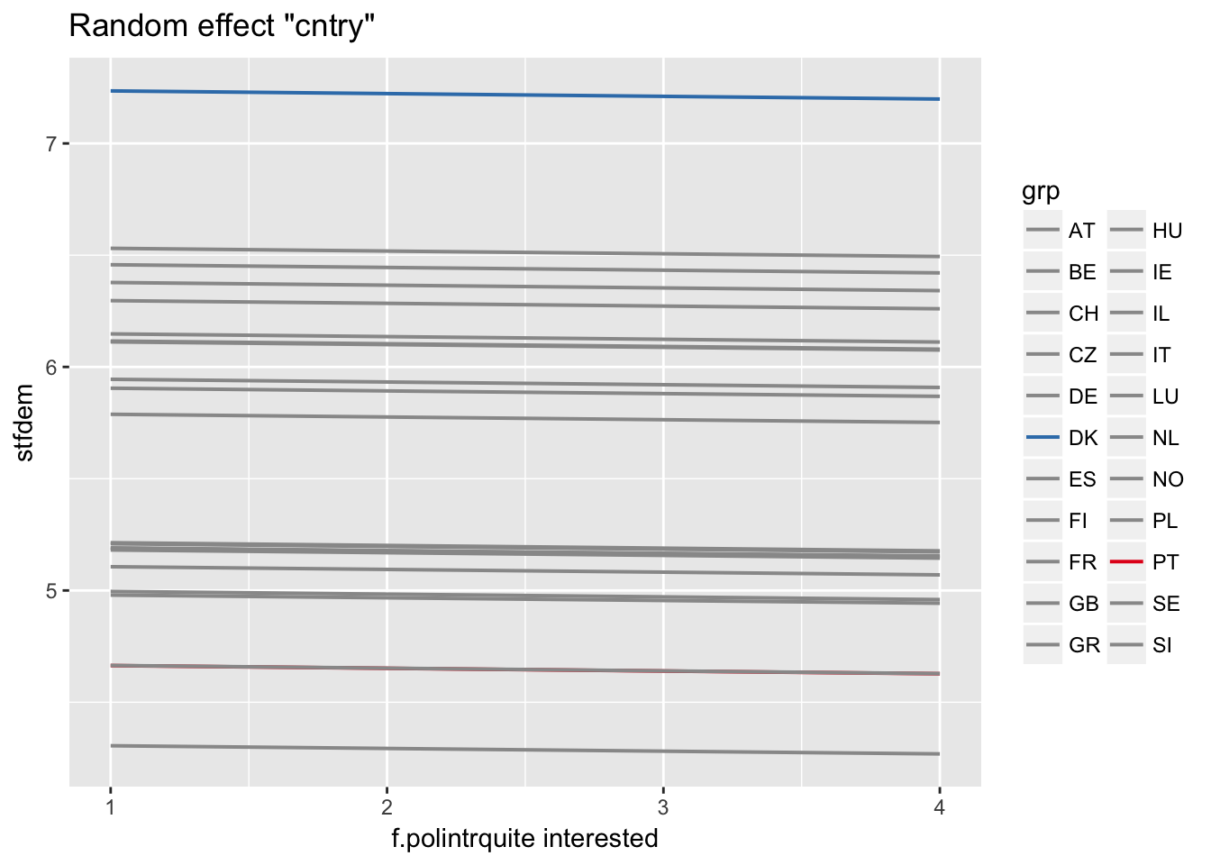
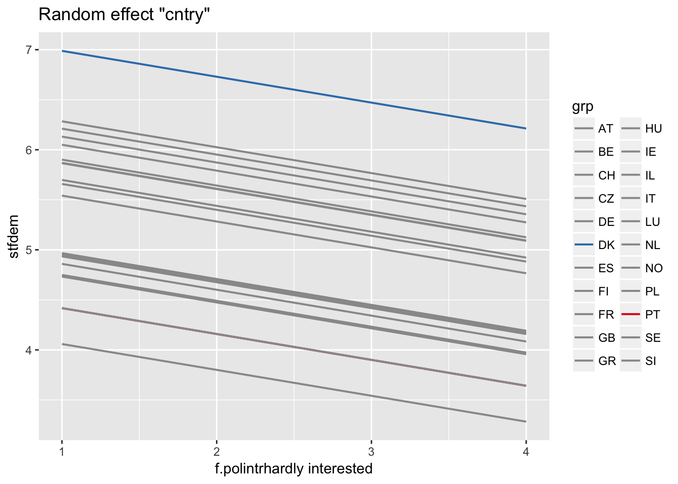
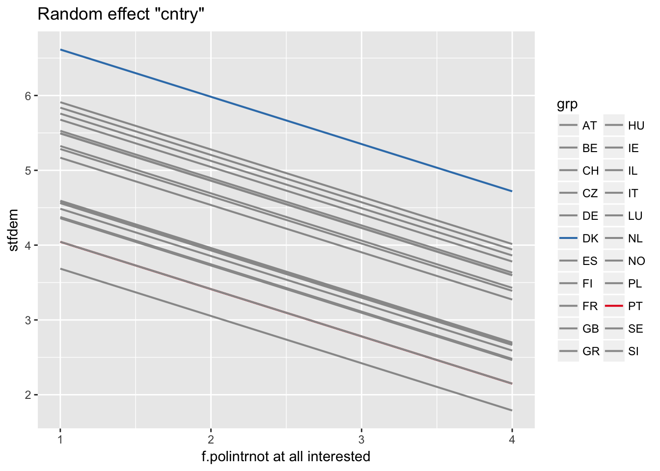
polintr | -.2396015 .0259574 -9.23 0.000 -.290477 -.188726
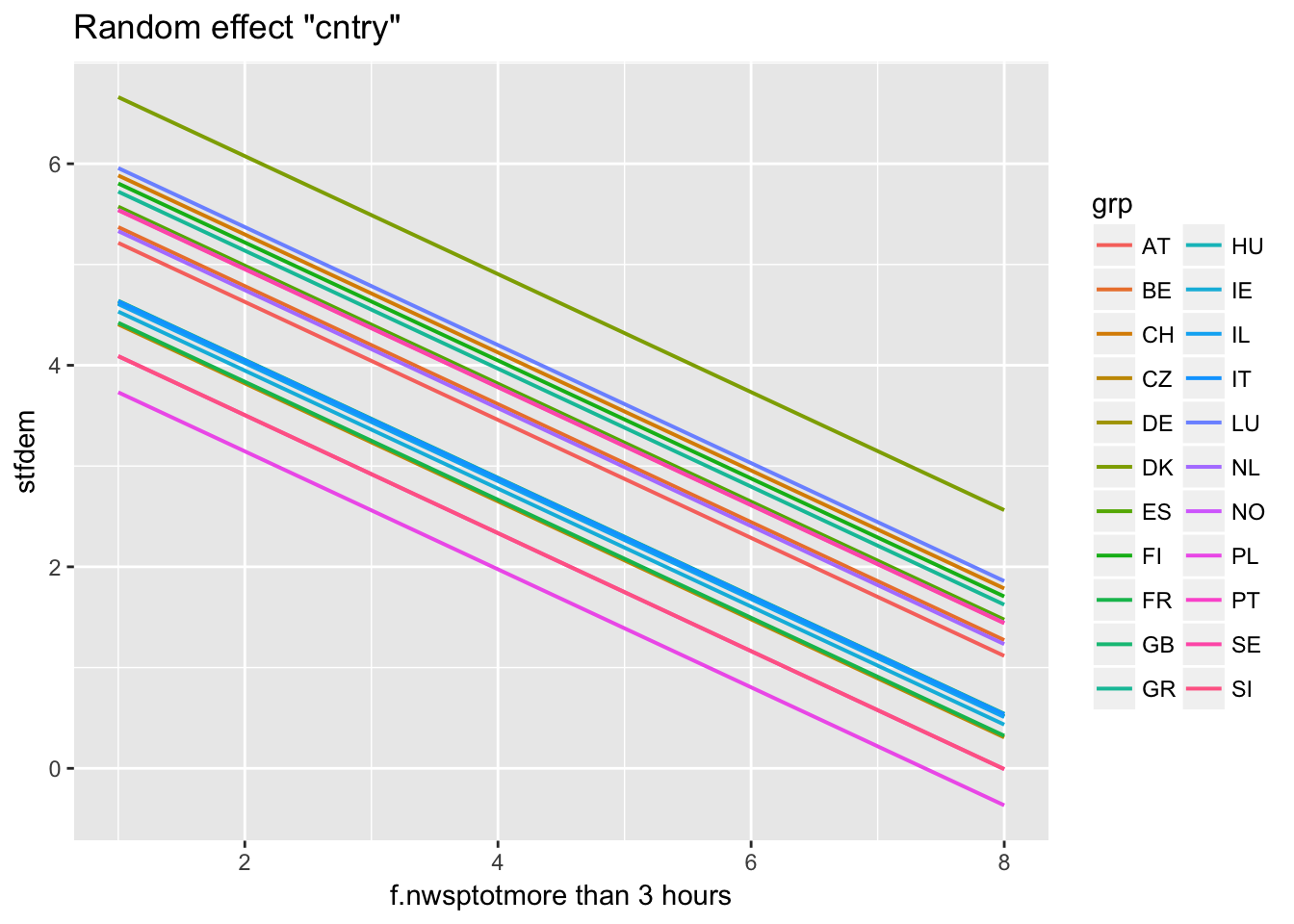
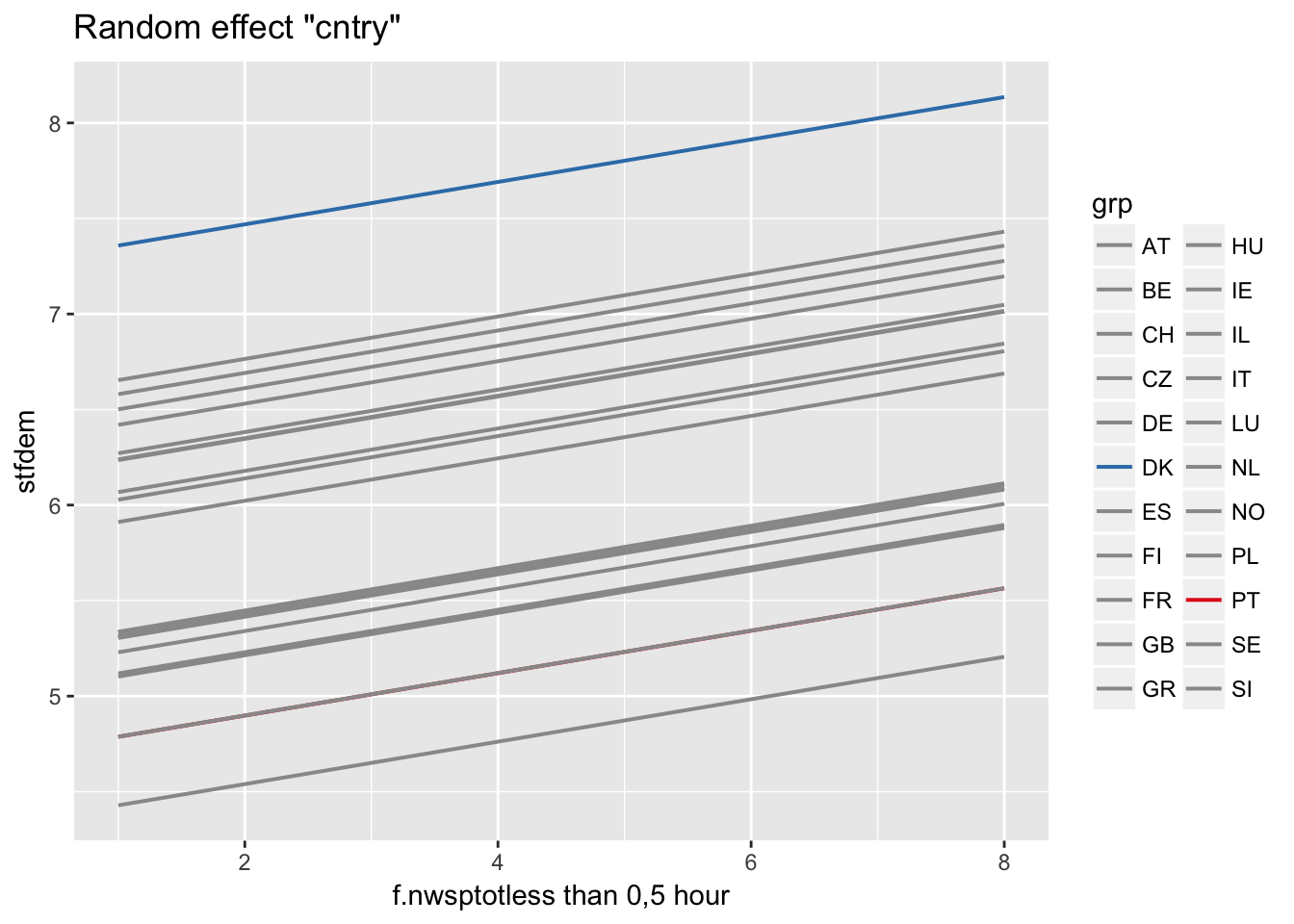
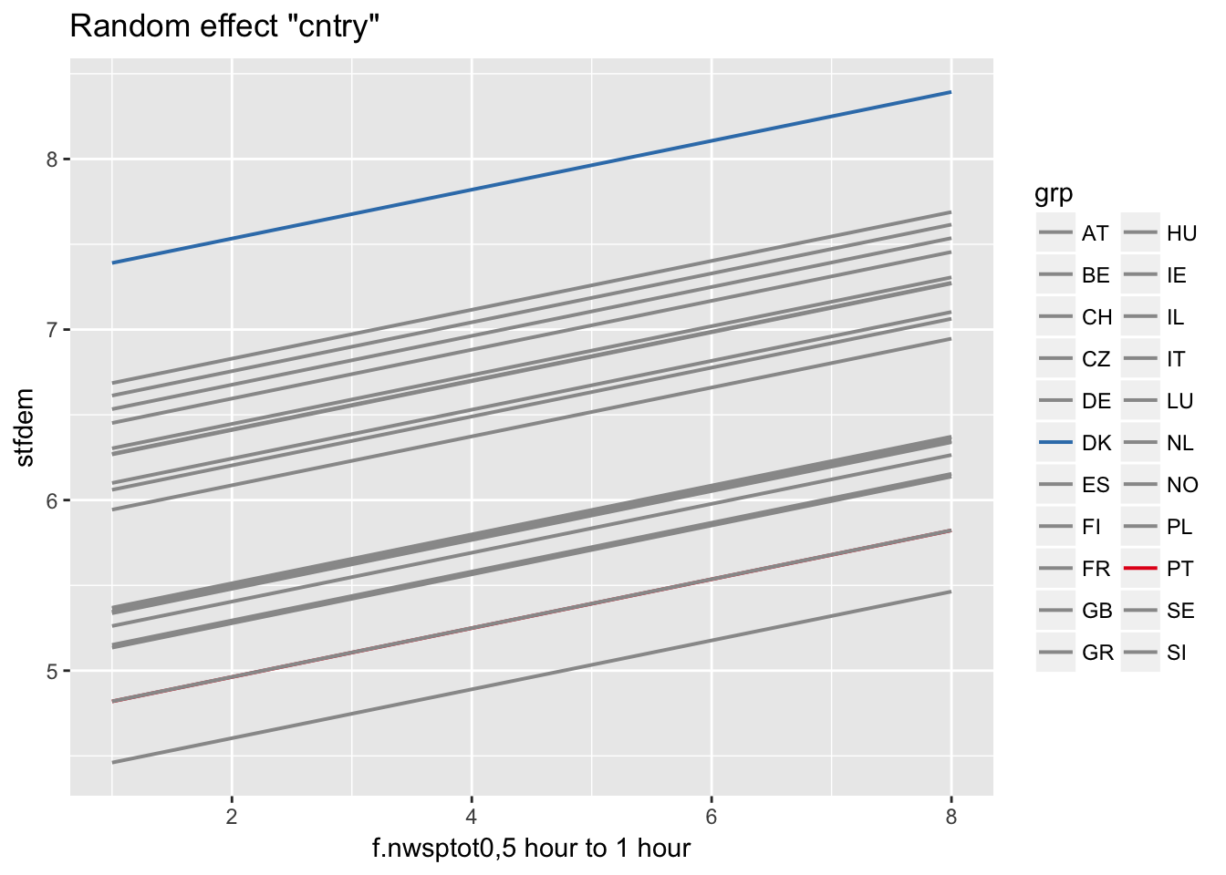
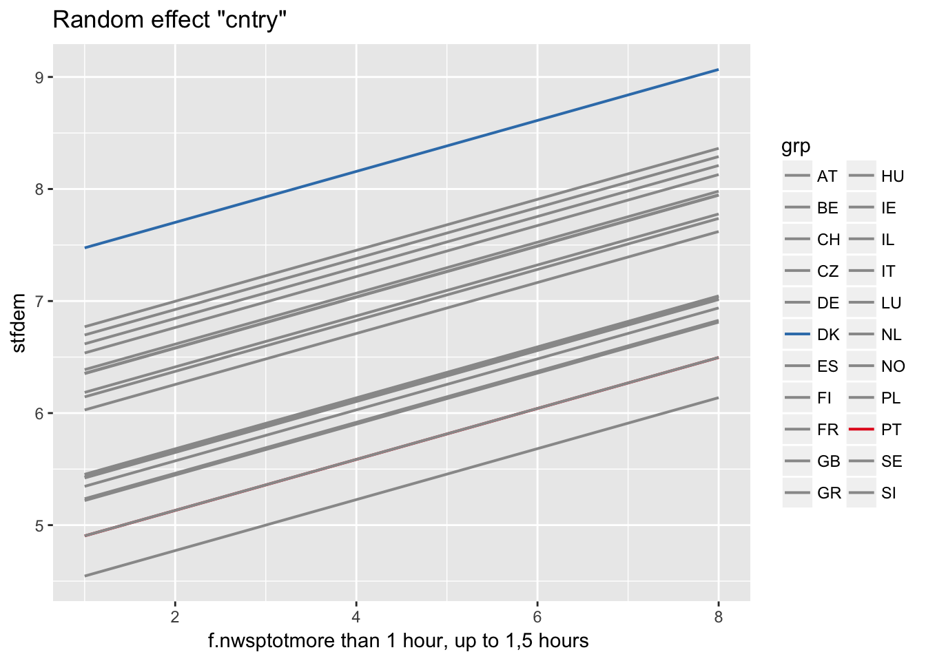
nwsptot | .006341 .0177099 0.36 0.720 -.0283696 .0410517
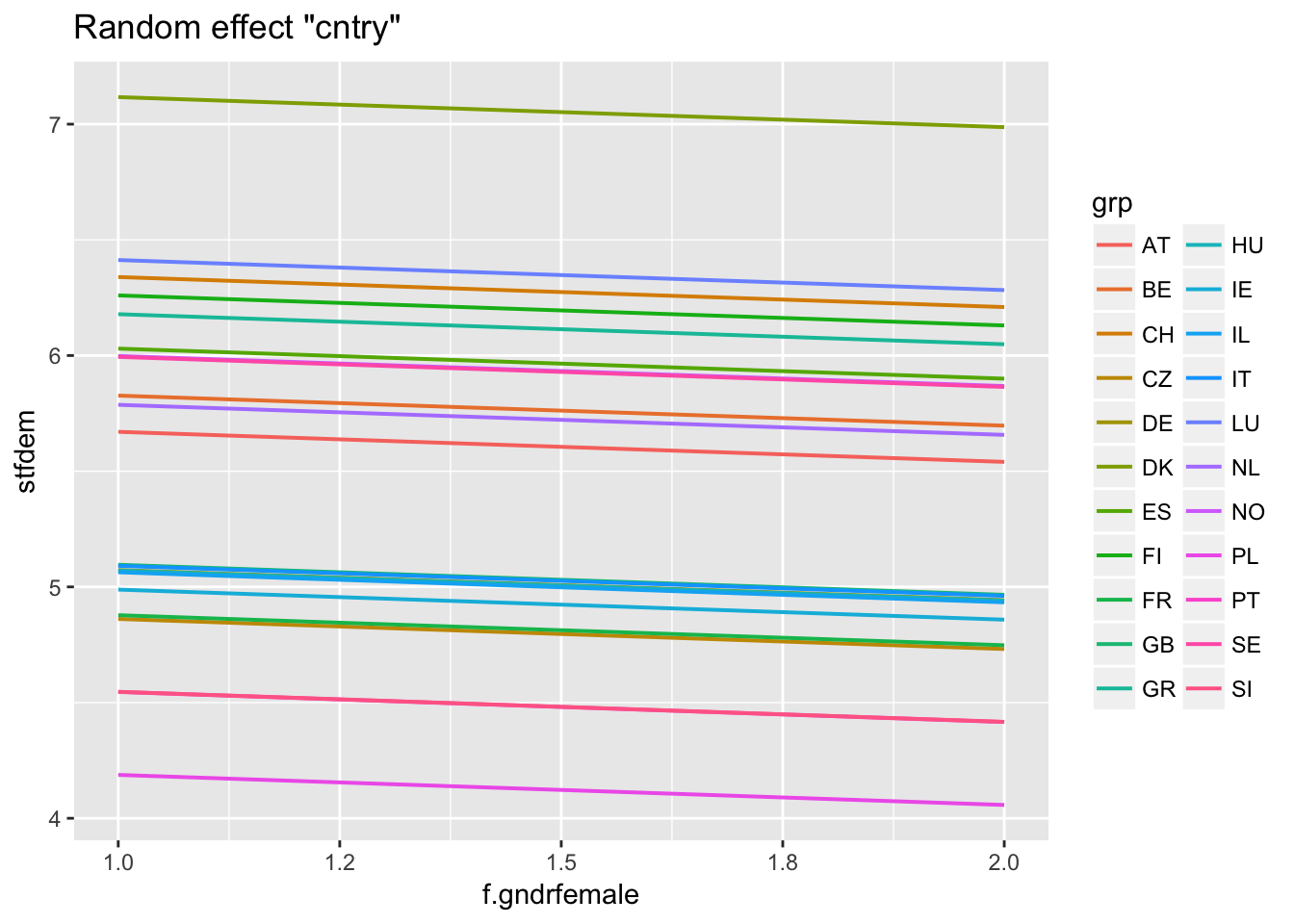
gndr | -.1248568 .0430147 -2.90 0.004 -.2091642 -.0405495
_cons | 6.253066 .1872712 33.39 0.000 5.886021 6.620111
------------------------------------------------------------------------------
------------------------------------------------------------------------------
Random-effects Parameters | Estimate Std. Err. [95% Conf. Interval]
-----------------------------+------------------------------------------------
cntry: Identity |
sd(_cons) | .7453428 .1158022 .5496761 1.01066
-----------------------------+------------------------------------------------
sd(Residual) | 2.214621 .0149712 2.185472 2.244159
------------------------------------------------------------------------------
LR test vs. linear model: chibar2(01) = 1089.47 Prob >= chibar2 = 0.0000
. estat icc
Residual intraclass correlation
------------------------------------------------------------------------------
Level | ICC Std. Err. [95% Conf. Interval]
-----------------------------+------------------------------------------------
cntry | .101745 .0284276 .0579964 .172453
------------------------------------------------------------------------------
R
First: Save Model (like Stata’s est store)
multi2 <- lmer(stfdem ~ polintr + nwsptot + gndr + (1|cntry), data = ess, REML = FALSE)
Then: Inspect model
tidy(multi2)
glance(multi2)
icc(multi2)
##
## Linear mixed model
## Family: gaussian (identity)
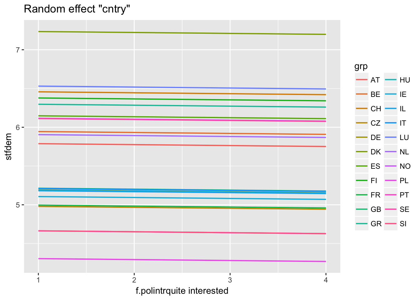
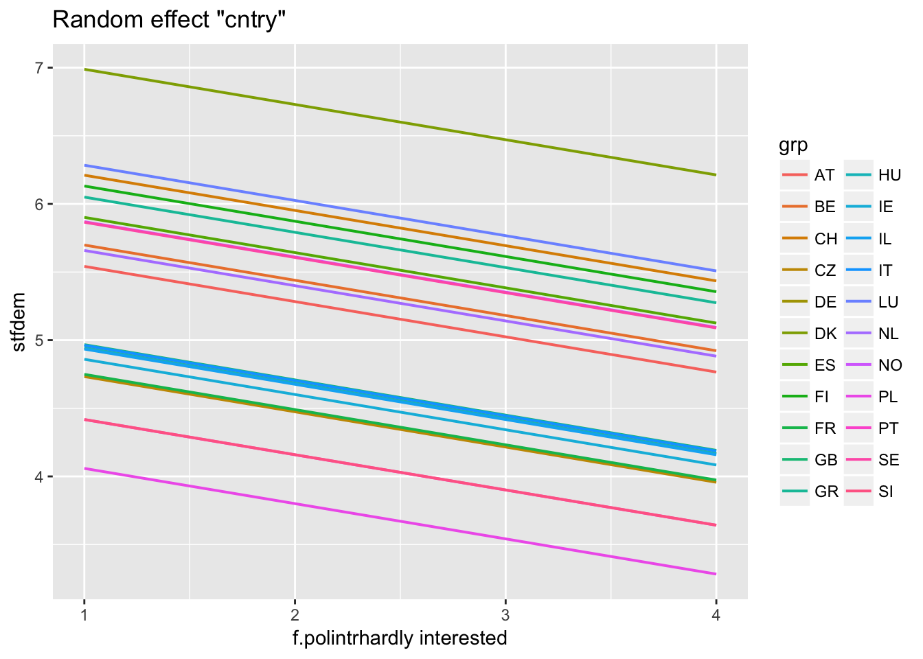
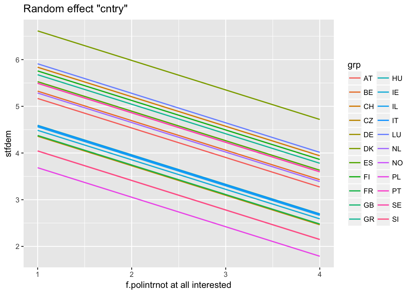
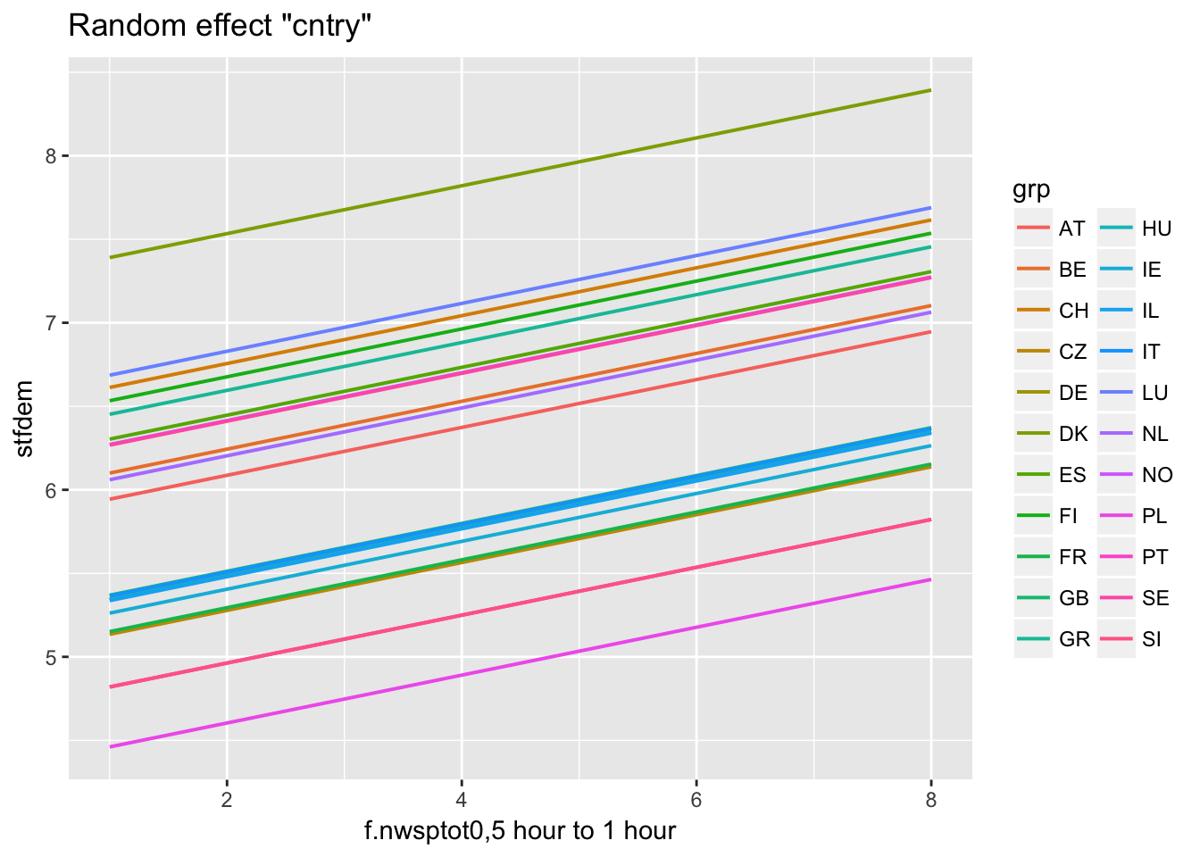
## Formula: stfdem ~ f.polintr + f.nwsptot + f.gndr + (1 | cntry)
##
## ICC (cntry): 0.100449
R-Squared, works for random intercept models only
r2(multi2)
##     R-squared: 0.1204
## Omega-squared: 0.1204
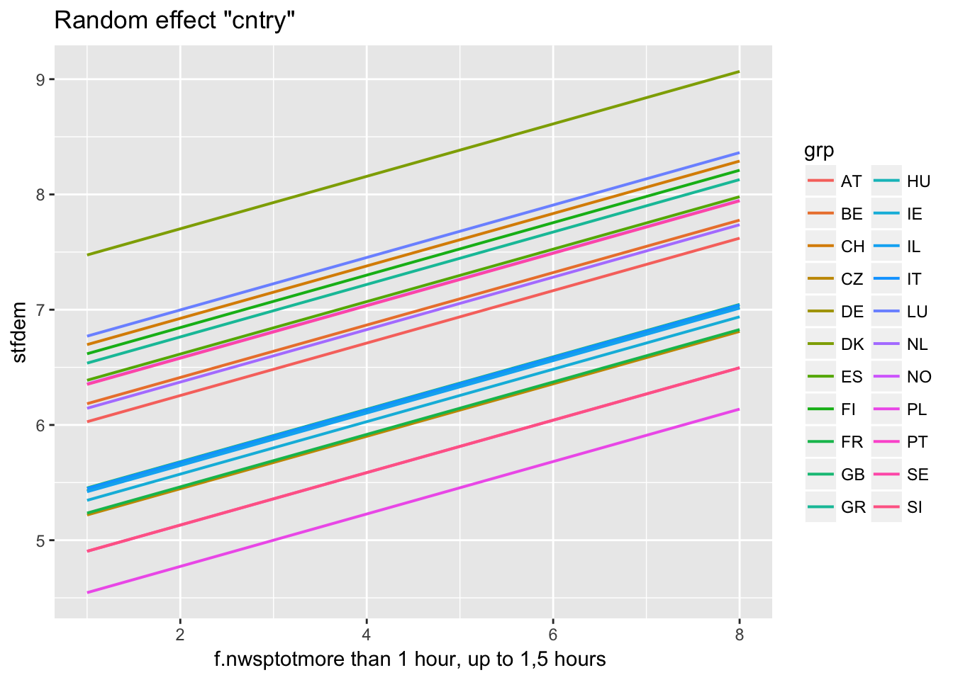
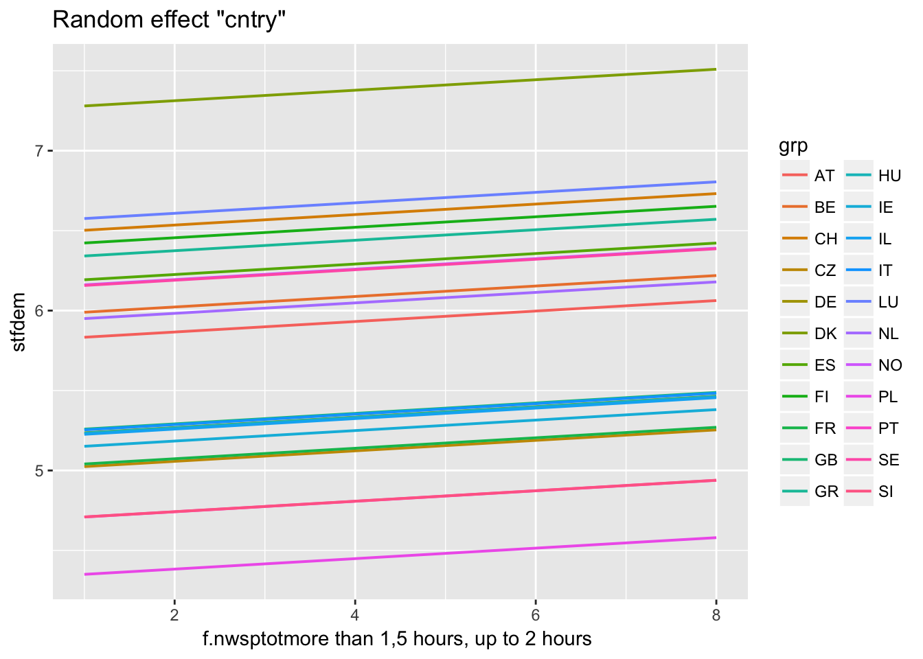
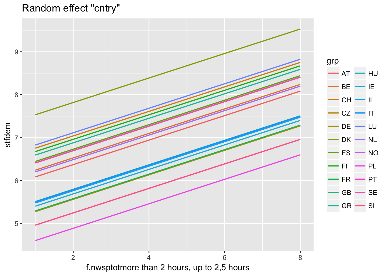
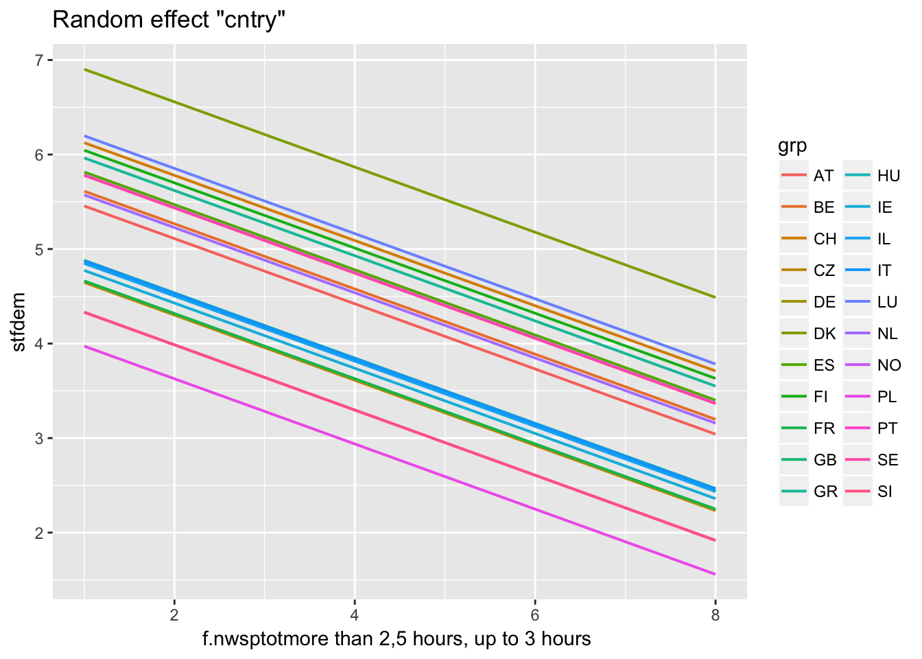
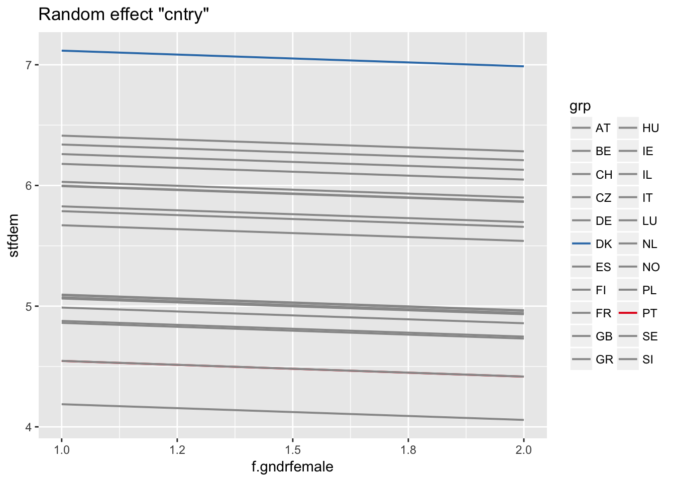
Predictions for individual cluster
ranef(multi2)
## $cntry
##    (Intercept)
## AT        0.17
## BE        0.33
## CH        0.84
## CZ       -0.64
## DE       -0.43
## DK        1.62
## ES        0.53
## FI        0.76
## FR       -0.62
## GB       -0.40
## GR        0.68
## HU       -0.43
## IE       -0.51
## IL       -0.44
## IT       -0.41
## LU        0.91
## NL        0.29
## NO        0.50
## PL       -1.31
## PT       -0.95
## SE        0.49
## SI       -0.95